Principal Component Analysis (PCA)
1 Continuous latent space
The idea is of latent variables is that the data is described in the low dimensional latent space and somehow it can map it to this hight dimensional space.
2 Principal Component Analysis (PCA)
Imagine I have the bottom right plot in multiple dimensions so not only 2D dimensions. I can compute a mean and a covariance matrix to fit this data.
Now I pick only line and I will fit the data in 1D-dimension i.e using Gaussian with the mean and convariance from the original plot. This mapping depends on the direction on the line for the PCA, imagine now the green line below then the gaussian will look different
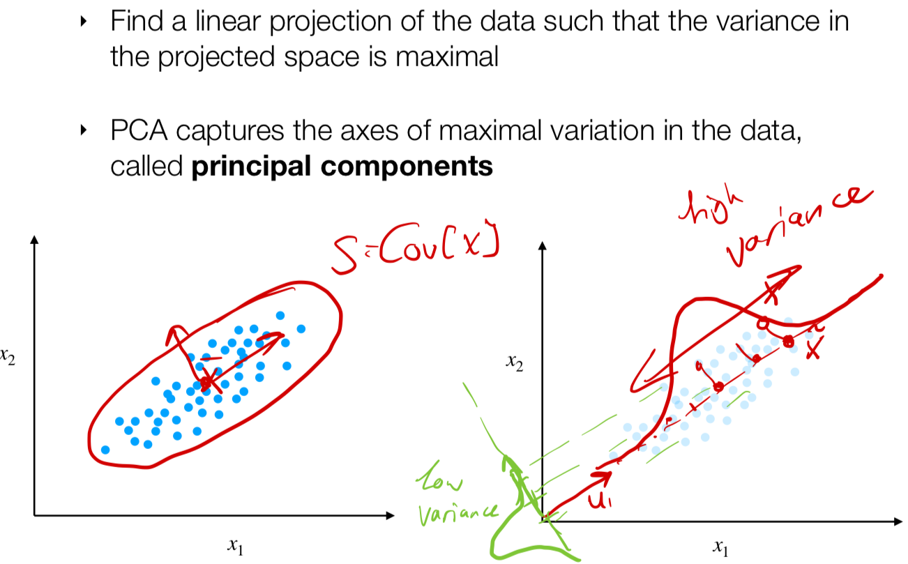
- So we want to find the direction in which it maximizes the variance data. This is important because if you have a low variance then all the points map to this compressed graph and may look like one point when in reality there are plenty.
3 Recall orthonomal projections
- The span of a vector.
4 1D Projection
Remarks:
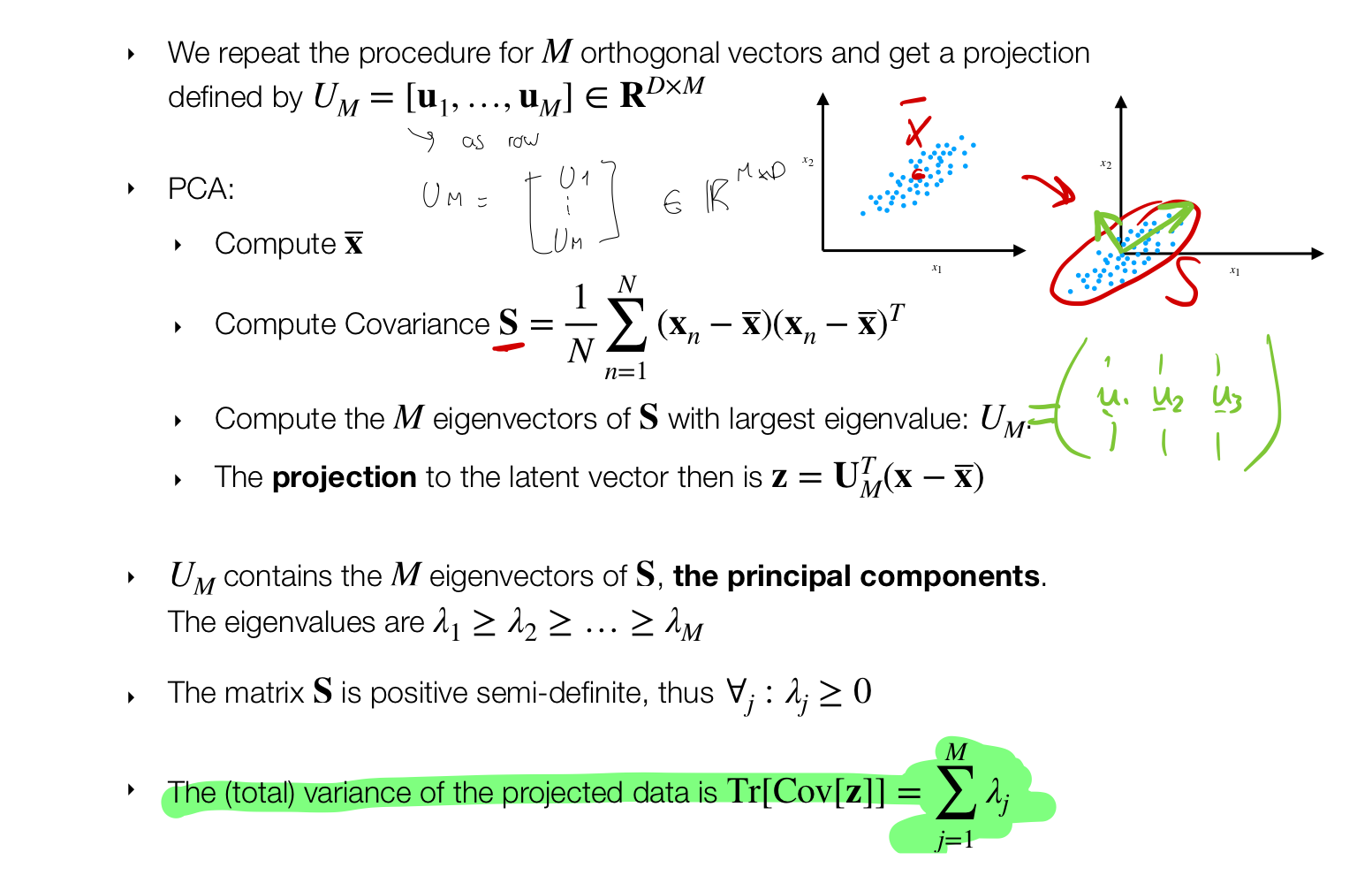
- Here the \(z_1\) is the projected point into the 1D-dimensional space if we would like more than one dimension then this z_1 would be now a vector \(\textbf{z}_1\) with dimensions \(M\)
5 Maximizing the variance of 1 component
The principal components are the \(u_1\) the lines (the directions)
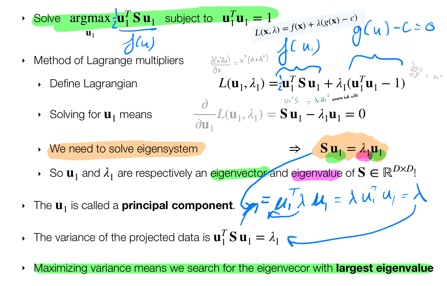
5.1 PCA via maximum variance
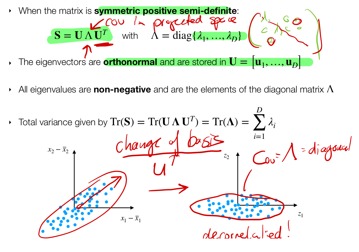
5.2 Reminder: eigen de-composition
Remarks:
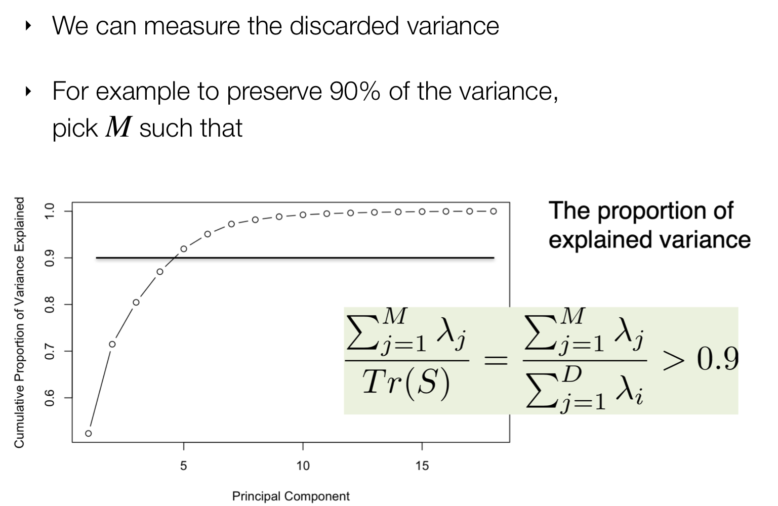
- The total variance of our datapoints in the new dimensional space can be calculated by summing up the eigenvalues
- We should think of \(U\) as a change of basis from the D-dimensional space to the new dimensional space. This new dimensional space its determined by how many eigevector at the end we choose
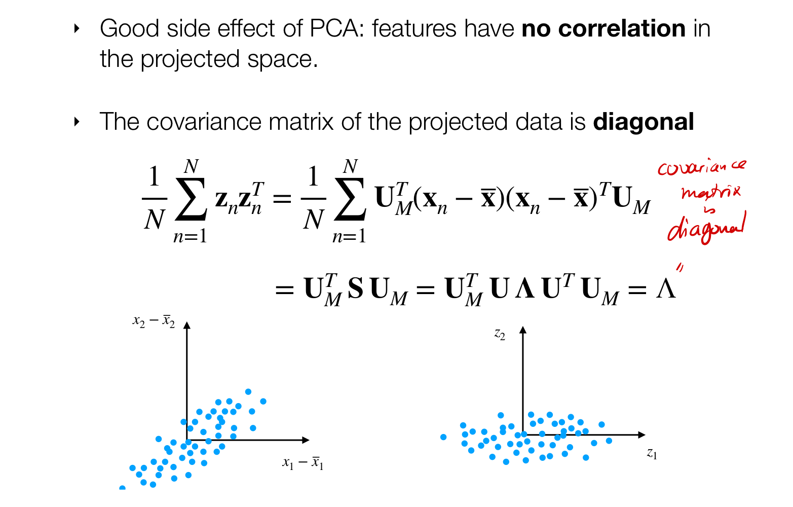
- Because the eigenvectors are orthonormal that means when we apply do the change of basis with the A_weird we are decorrelating our data.
5.3 How to choose M?
5.4 Feature Decorrelation
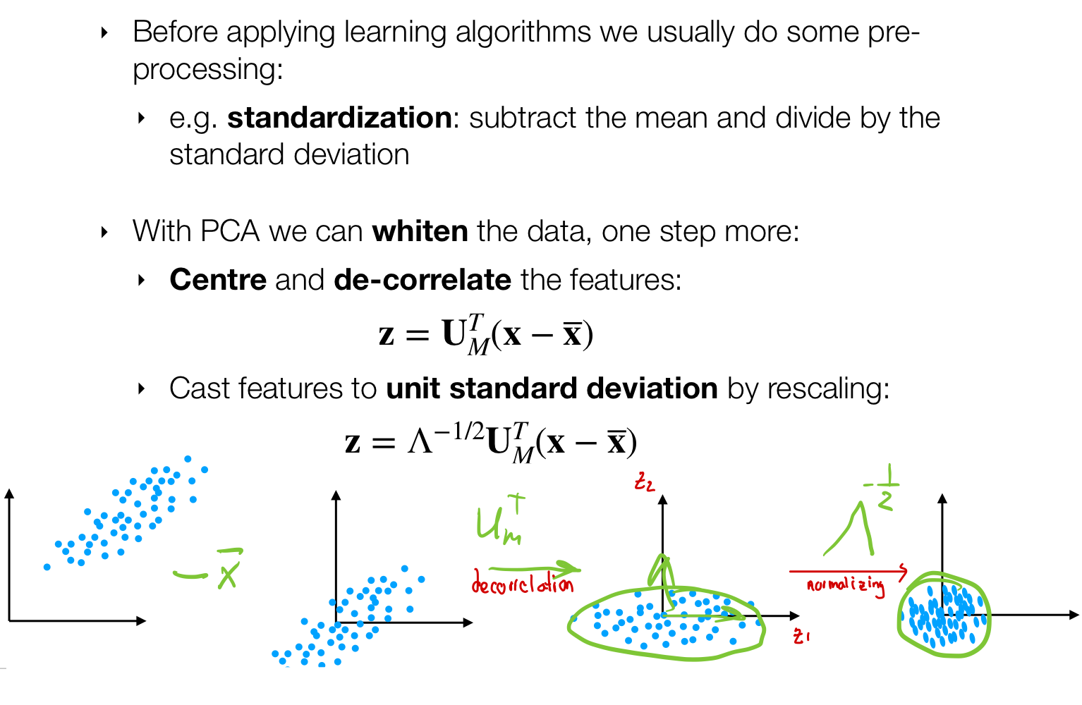
5.5 Applications: Whitening
6 Probabilistic PCA
- Discrete latent models: k-means, Gaussian Mixture models
- Continuous latent models: probabilistic PCA, unsupervised regression
If you compare k-means as latent clarifier then this can be consider as an unsupervised regression
If you compare Gaussian-mixture model then this can be though as continuous PPCA model
Probabilistic view of PCA:
- Learn it via maximum likelihood
- (Third) alternative view of PCA
- Both latent and observed variables are Gaussian
6.1 Continuous latent variable model
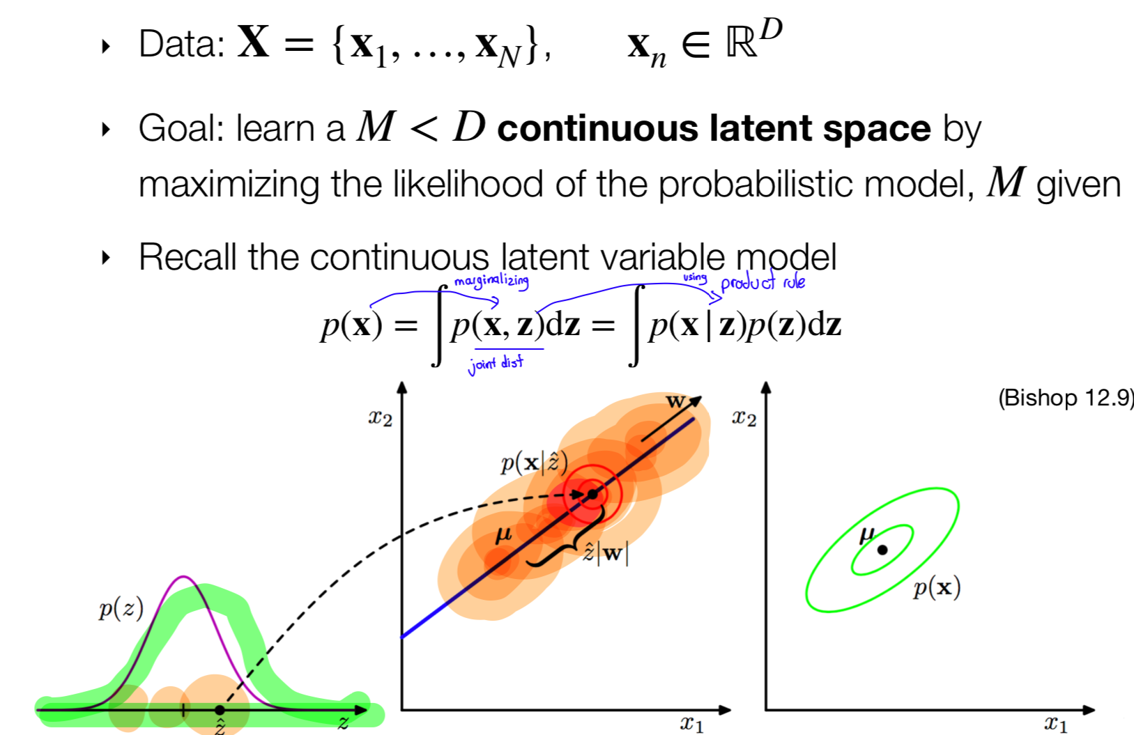
- We assume that there is a latent space z from which we can sample a point z.
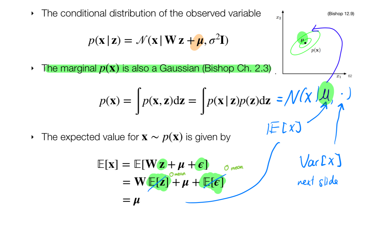
- Then I have this conditional p(x|z) given z what is the probability that is lands
6.2 PPCA modelling assumptions
Recall z was the latent variable, the hidden variable the one its making something that we have x. Remember toughs –> words
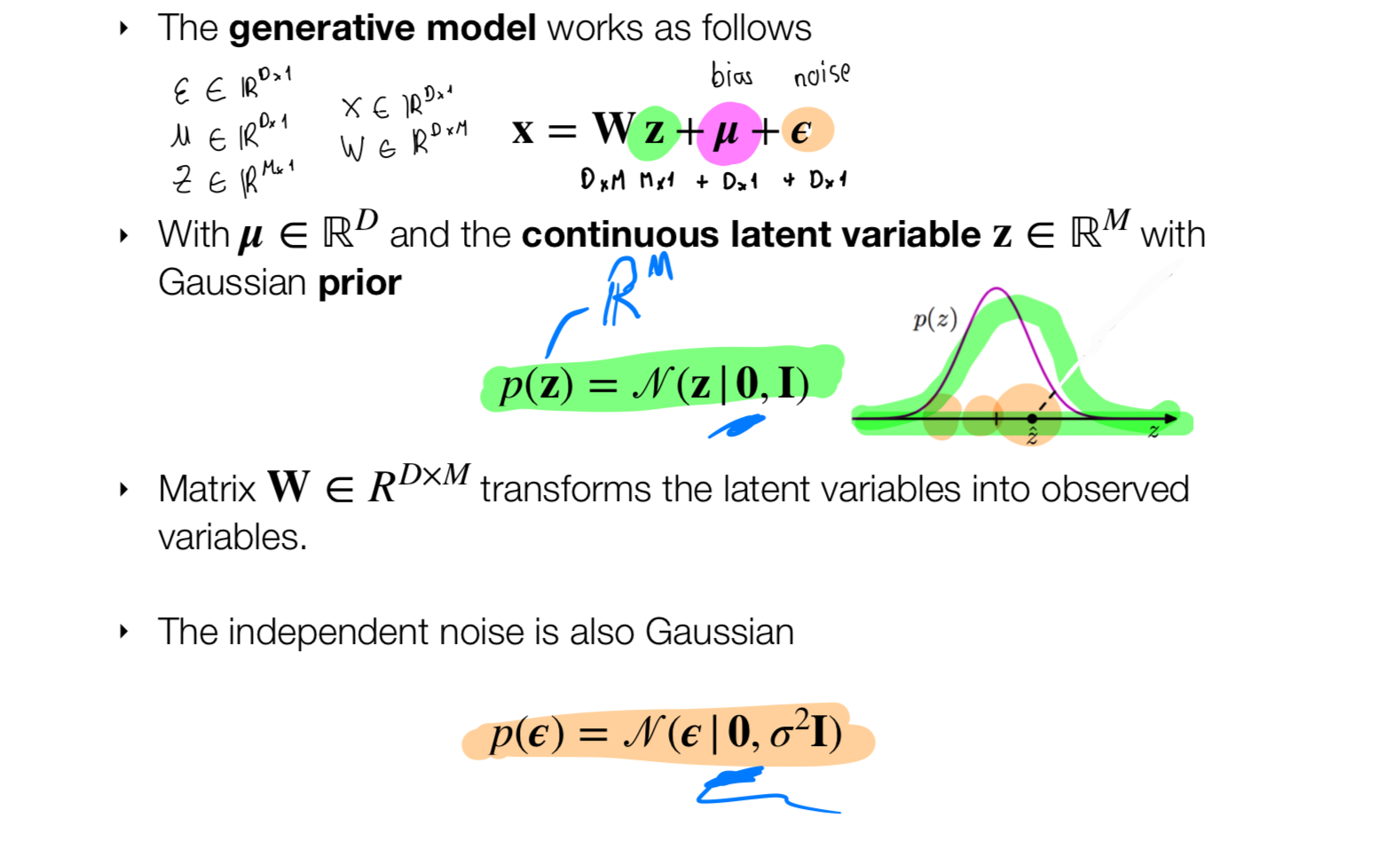
- We assume that x is formed by a linear combinations with the latent variable z, W, \(\mu\) and \(\epsilon\)
- Here we are saying that there is a linear relation between z and x.
- Here we are saying that there is a linear relation between z and x.
- Here, \(W\), \(\mu\) and \(\epsilon\) are the parameters that we want to recover
- Because z is Gaussian and noise is also modelled by Gaussian, then \(x\) will also be Gaussian
6.3 It follows
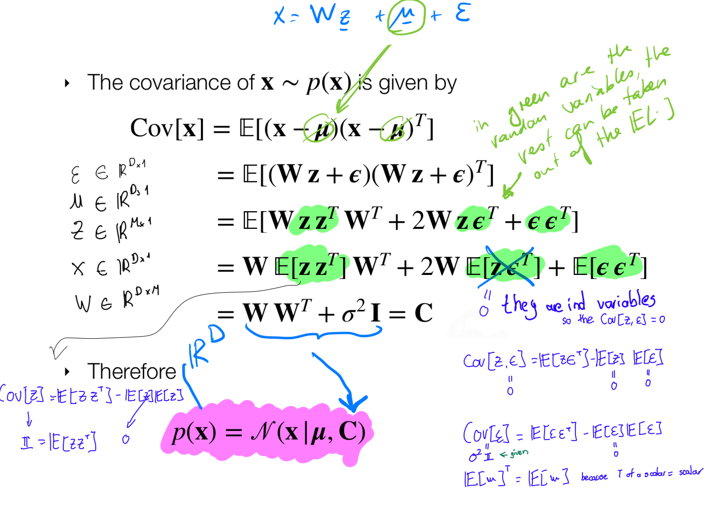
- In the covariance part we take out W because its not a random variable
6.4 Probabilistic PCA in a picture
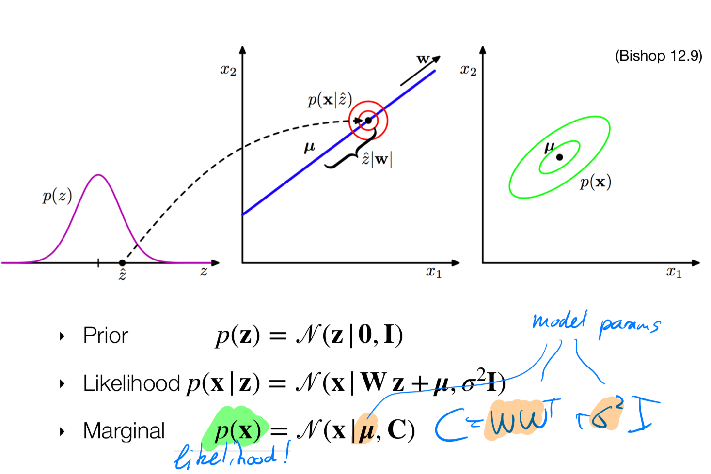
From now on we can find the parameters by doing MLE
6.5 The log-likelihood
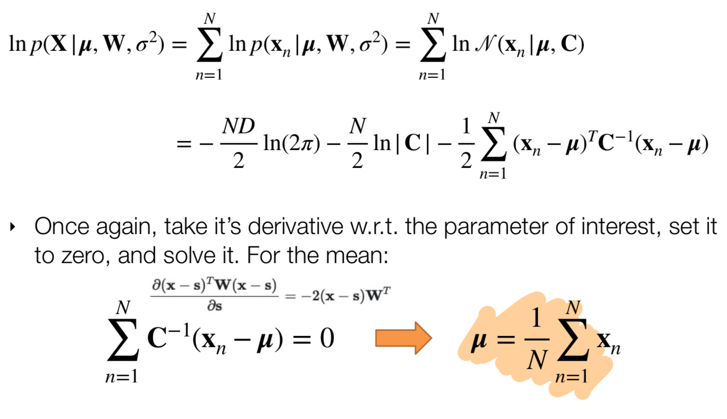
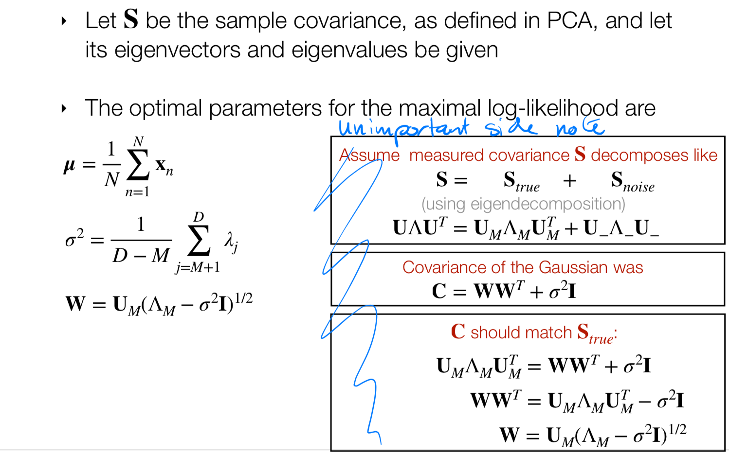
6.6 PPCA has closed-form solutions
6.7 PPCA Summary
Three views:
- Max variance, min reconstruction error, probabilistic
Applications
- Dimensionality reduction
- 2D/3D visualization
- Compression
- Whitening (de-correlating features)
- (not mentioned) De-noising: discard the smallest variance features = the noise components (hopefully!)
Limitations:
- Only linear transformations
6.8 Comparing PCA & PPCA
The PCA can be expressed as the maximum likelihood solution probabilistic PCA.
Advantages of the probabilistic PCA over the conventional PCA:
- We can associate a likelihood function to the probabilistic PCA which allows a direct comparison with other probabilistic density models
- Probabilistic PCA can be used to model class-conditional densities and can thus be used in classification problems
- We can run the model generatively to provide samples from the modeled distribution.
7 Non Linear PCA
Find the subspace that maximizes the variance of the projection or minimizes the reconstruction error
By linear we mean all the data is cluster around one contour line like the green line. The question is can we do non-linear PCA where we have not the reed line which is clearly non-linear?
8 PCA using basis functions
The question is how do we map these non-linear data to a linear line such that we use basis function. We can do this in two ways:
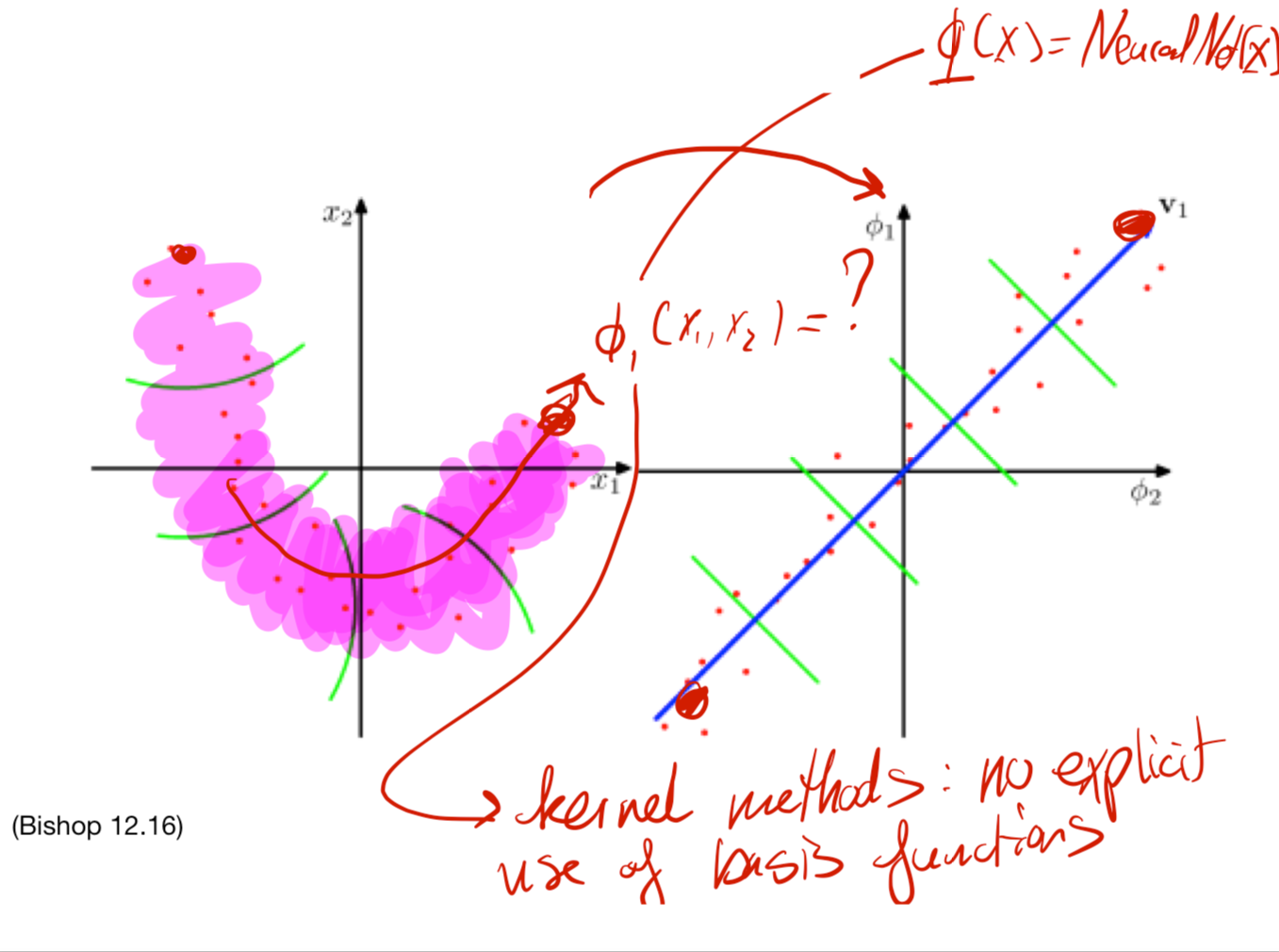
- Using Neural Networks
- Using kernel methods: we can do the mapping from original space to the new space without explicit modeling the basis functions
- We can use Neural Networks. For instance \(\mathbf{\phi(\textbf{x})} = NN(\textbf{x})\), where \(\textbf{x}\) is the input vector
- We can use Kernel methods where we do not make explicit use of basis functions
We will first sketch the structure of an autoencoder
9 Auto-encoders (auto-associative neural nets)
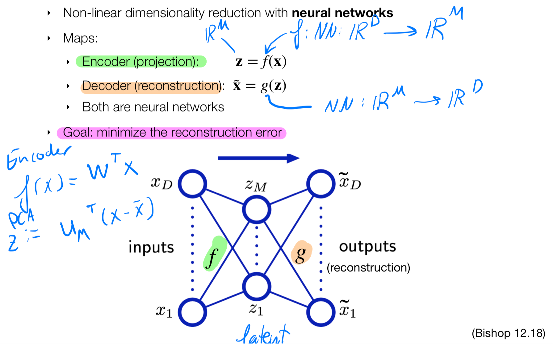
If \(f(x)=w^Tx\) is a linear projection that goes from D to M then this resembles to PCA where we have \(z=\mu_M^T(x-\bar x)\). So if the function \(f(x)\) is of form like in the PCA case then we have a linear projection that can transform our points to a lower dimensional space
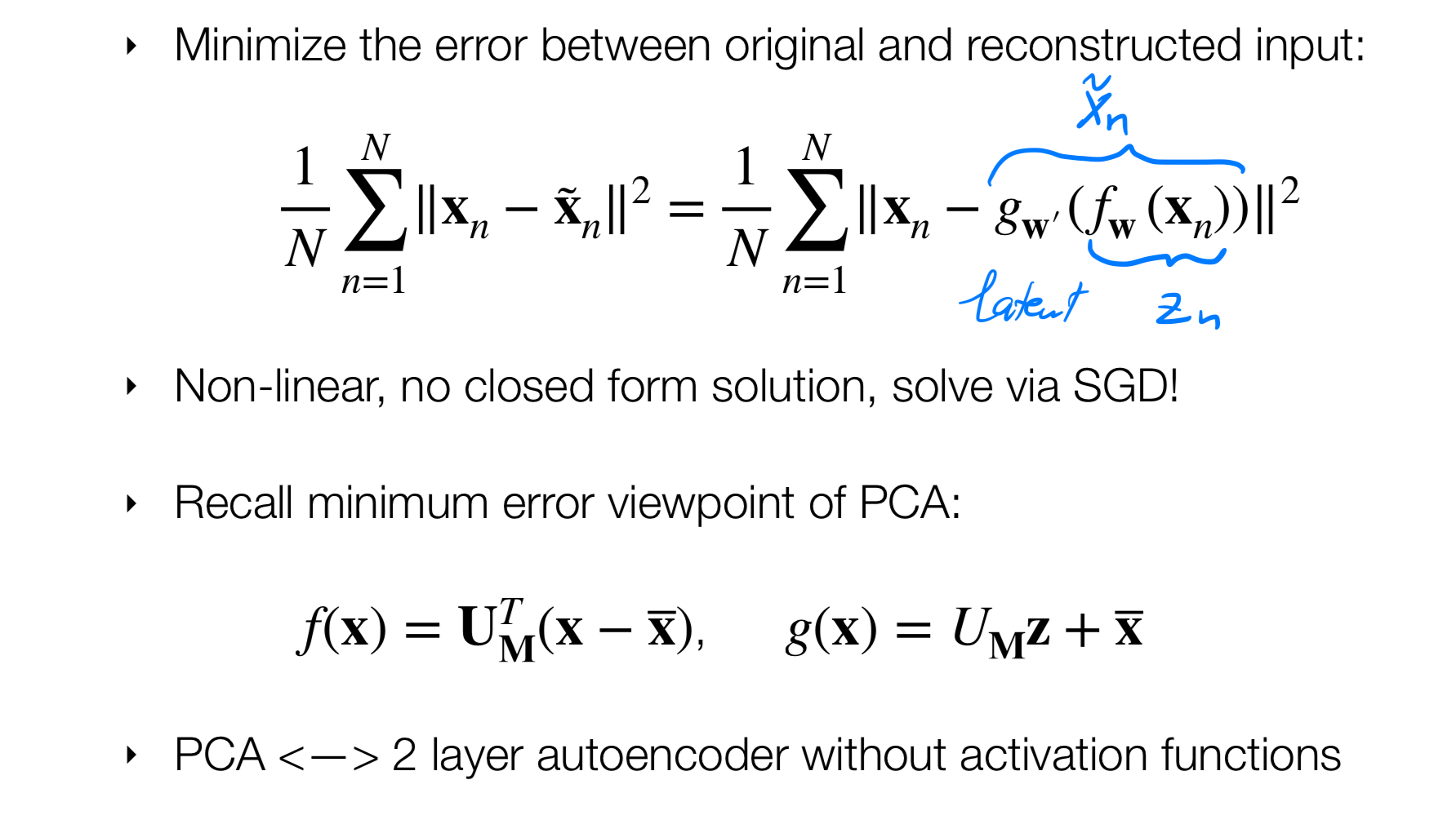
10 Autoencoder objective
- The mapping from input through the encoder, we call it the latent \(z_n\). The later is like a compression.
- Before we will project the data into our principal components but now we let the NN learn what the latent mapping should be
- When we carry out this encoder and decoder without using activation functions we end up in the PCA structure
- If we use however activation function and we use more layers than 2, then we have a non-linear model which has no closed solutions and therefore we can solve it by SGD because our error is non-convex
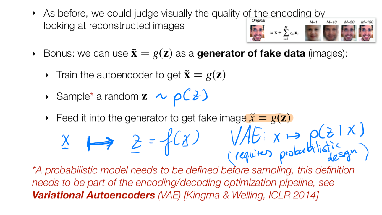
11 Autoencoder as generator
12 Kernel PCA
We are use to express things in terms of features vectors, i.e the latent is obtained by taking the features vectors and projecting it onto a lower dimensional space
Now we are going to report our results in terms of the kernel \(k(\textbf{x}\textbf{x}_n)\). The result is that the projection would be purely in terms of the other data points via the kernel but not by my other parameters
This is another way how to do PCA for non-linear