Recall: Variance measures the variation of a single random variable (like the height of a person in a population), whereas covariance is a measure of how much two random variables vary together (like the height of a person and the weight of a person in a population)
In a 2D dimensional feature space with 10 data points, the covariance matrix provides a measure of the relationship between the two features (dimensions) and how they vary together. The covariance matrix is a 2x2 matrix that quantifies the degree to which the two features change together
Let’s say you have two features, \(\textbf{x}\) and \(\textbf{y}\), and you have 10 data points with values (x_1, y_1), (x_2, y_2), …, (x_10, y_10). The covariance matrix Σ is calculated as:
cov(\(\textbf{x}\), \(\textbf{x}\)) is the covariance between feature \(\textbf{x}\) and itself (the variance of \(\textbf{x}\)).
cov(\(\textbf{y}\), \(\textbf{y}\)) is the covariance between feature \(\textbf{y}\) and itself (the variance of \(\textbf{y}\)).
cov(\(\textbf{x}\), \(\textbf{y}\)) and cov(\(\textbf{y}\), \(\textbf{x}\)) are the covariances between feature \(\textbf{x}\) and feature \(\textbf{y}\).
The covariances of two random variables (the two features) are calculated using the formula:
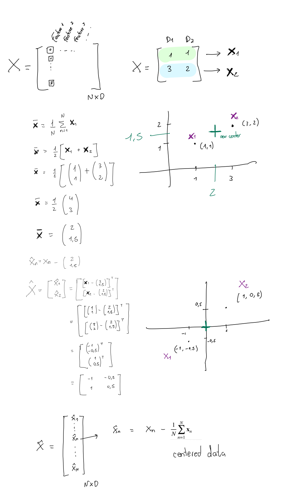
\(\textbf{x}_n \in \mathbb{R}^{Dx1}\) where \(D\) is the number of features (or number of dimensions i.e. with two features then 2-dimensions, with three features 3-dimensions)
\(\mathbf{\bar{x}} \in \mathbb{R}^{Dx1}\)
Below some example:
1 Python Example
Code
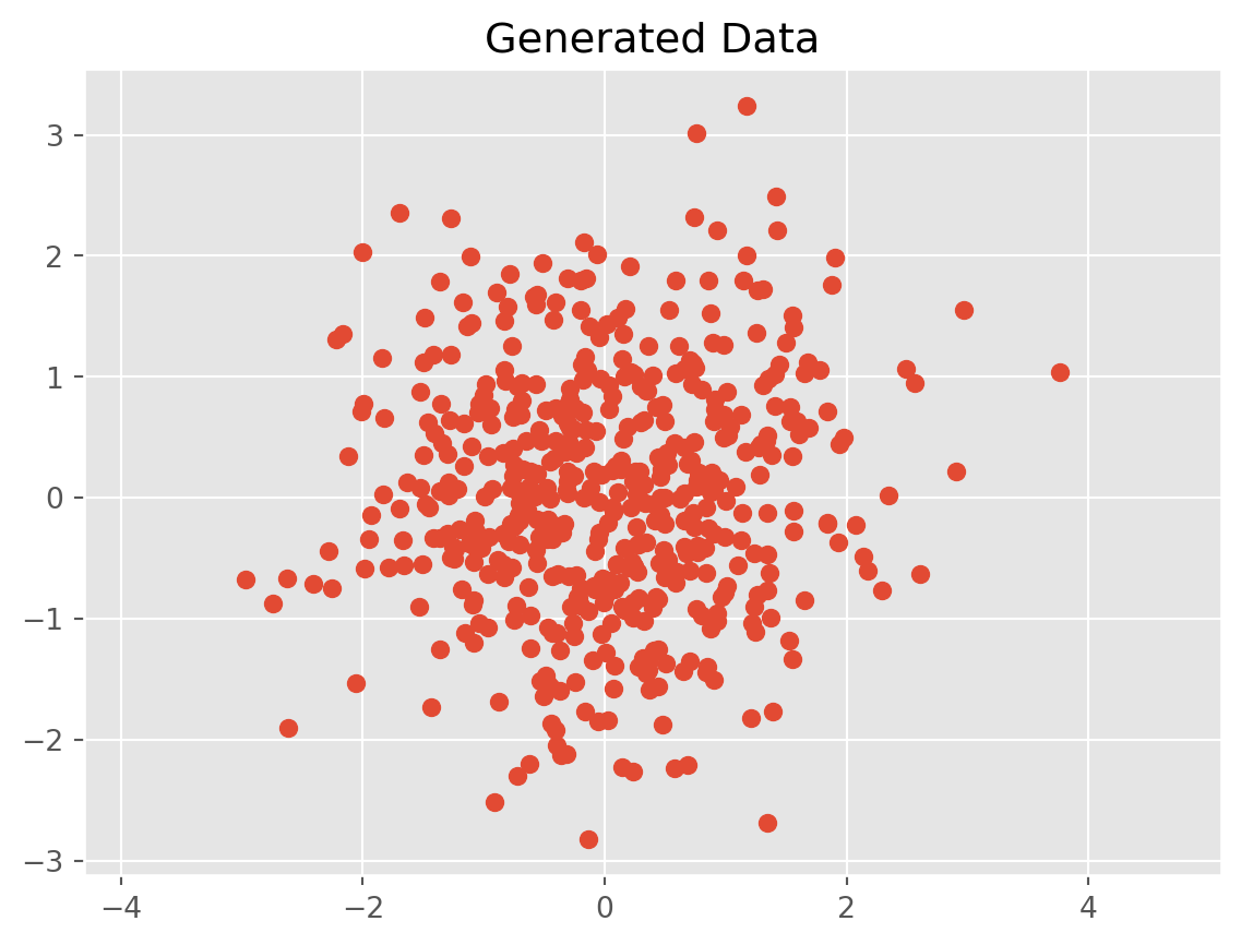
import numpy as npimport matplotlib.pyplot as plt%matplotlib inlineplt.style.use('ggplot')# plt.rcParams['figure.figsize'] = (12, 8)# Normal distributed x and y vector with mean 0 and standard deviation 1x = np.random.normal(0, 1, 500)y = np.random.normal(0, 1, 500)X = np.vstack((x, y)).Tplt.scatter(X[:, 0], X[:, 1])plt.title('Generated Data')plt.axis('equal')plt.show()
If two feature vectors are independent (or uncorrelated) the matrix matrix would be:
If this data was generated with unit cov(x,x) and unit cov(y,y) then we have a Identity covariance matrix
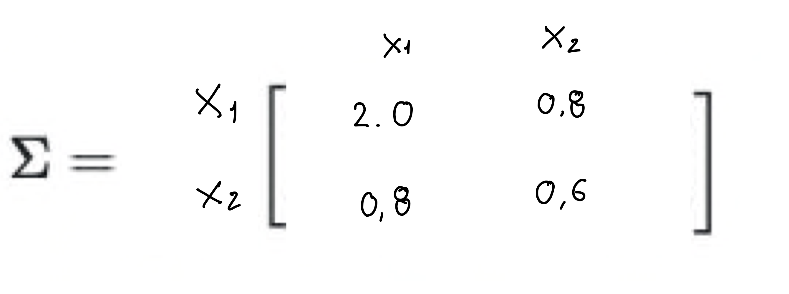
As x1 increases x2 increases too, because we have 0.8. We have a positive correlation on the data.
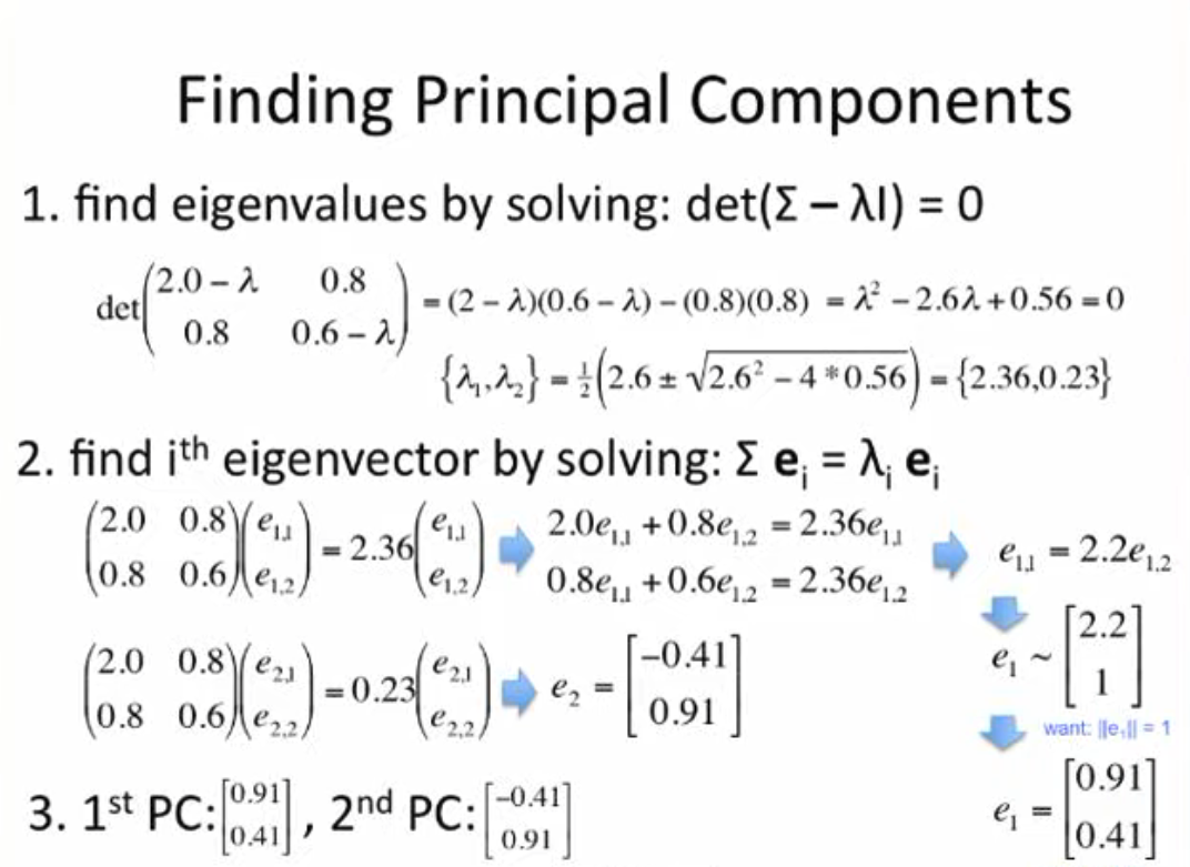
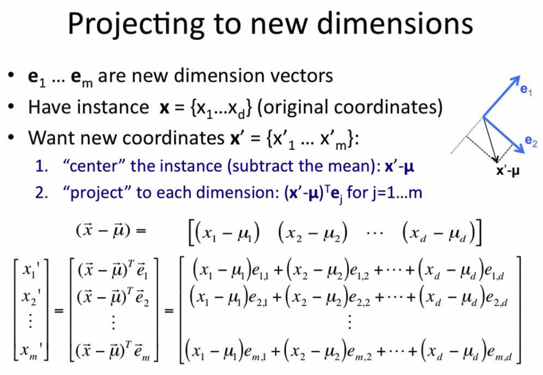
2 Relation with PCA
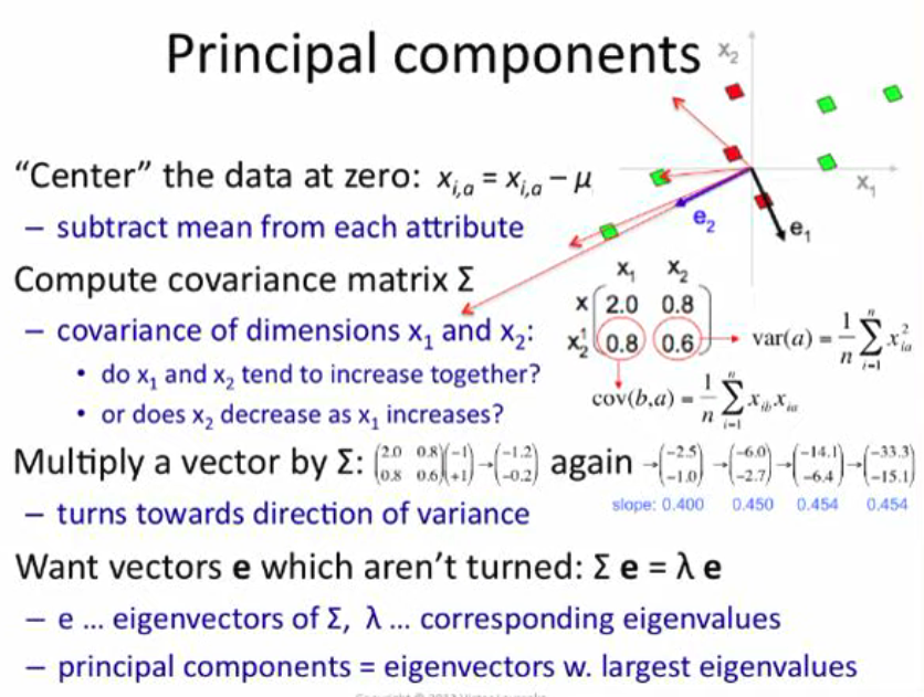
When you multiply the \(\Sigma\) covariance matrix times a vector and then again and again you end up with a vector that points to directions where you have the greatest variance in the data. So like where all points are spread out.
If I multiply the vector \(e2\) by the cov matrix it will not turn but will get longer and longer but will point in the same direction
Thus we want to find some vector \(e\) that when we multiply it with the cov matrix do not change direction. The vectors are called eigenvectors and the lambdas so the scalar version will be called eigenvalues.
The later point will be called our principal components which are the eigenvectors with the largest eigenvalues