Deep Feedforward Networks
1 From linear functions to nonlinear = from shallow to deep
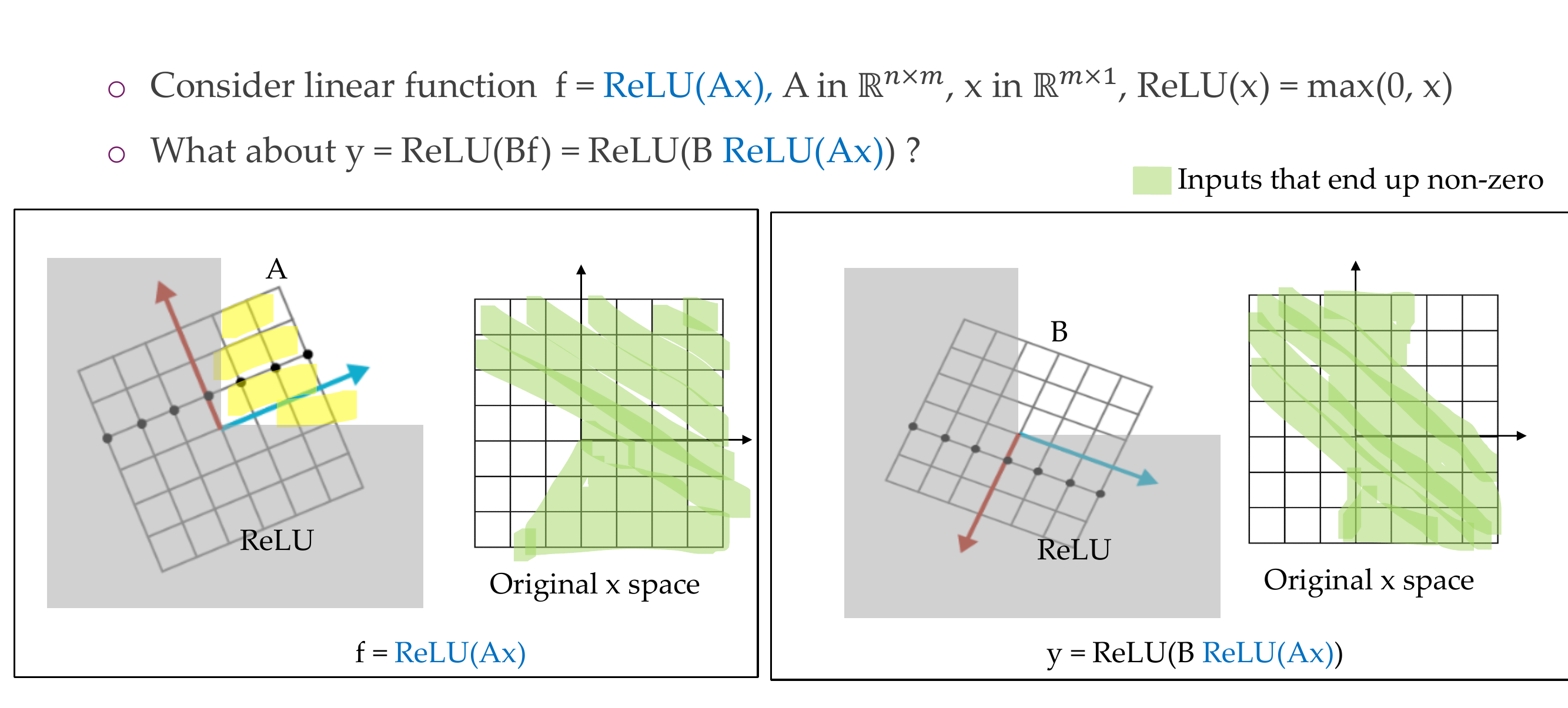
Here to apply first a Relu and the output of that another Relu: \(\sigma(B\sigma(A\textbf{x}))\)
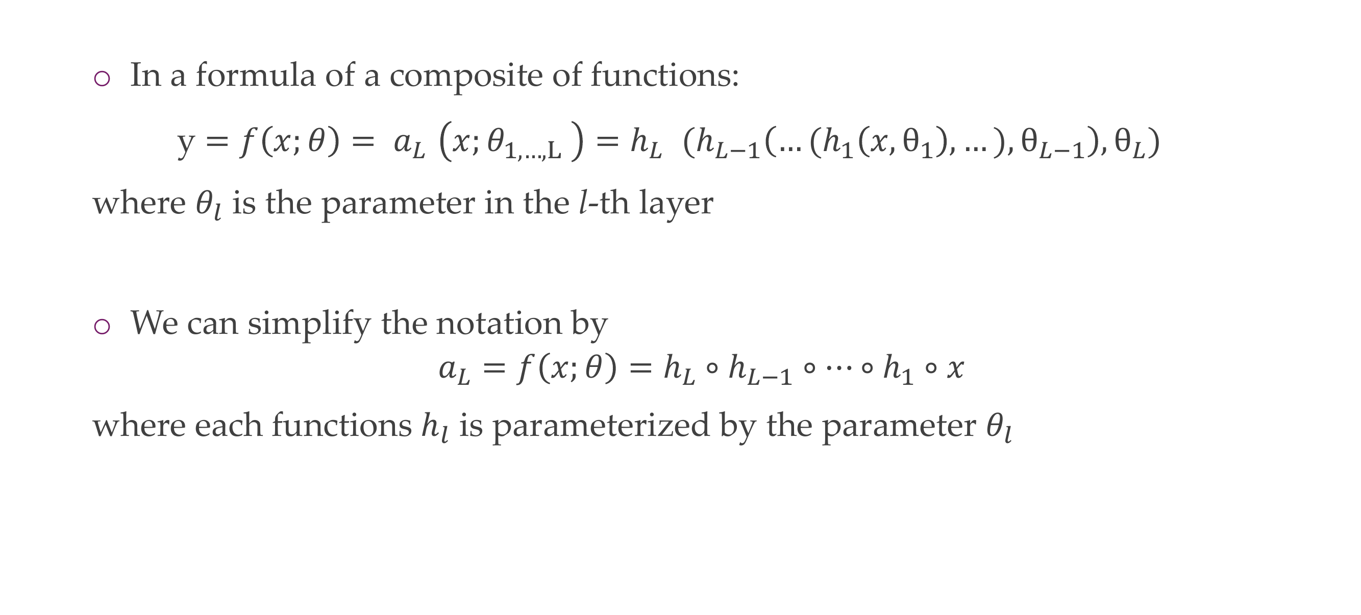
2 Deep feedforward networks
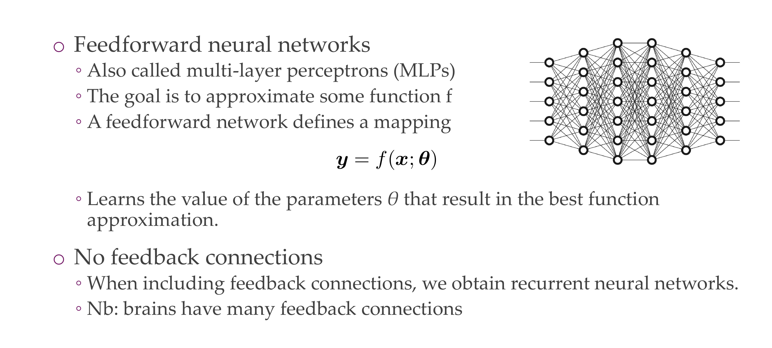
MLP is just a combination of multiple linear perceptrons, in each layer there would be parameters ie \(A\) is \(\theta_1\), \(B\) is \(\theta_2\)
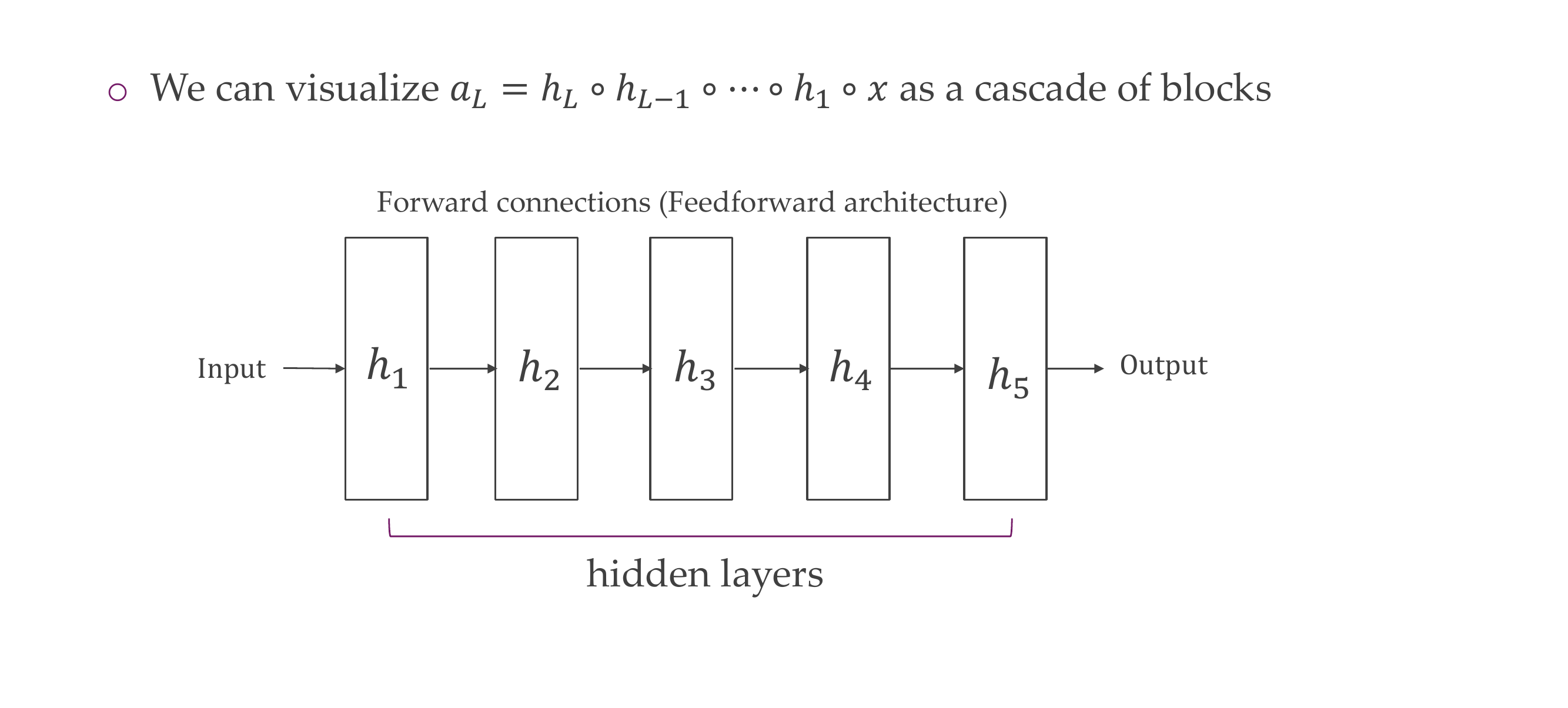
3 Neural networks in blocks
4 Non-linear feature learning perspective
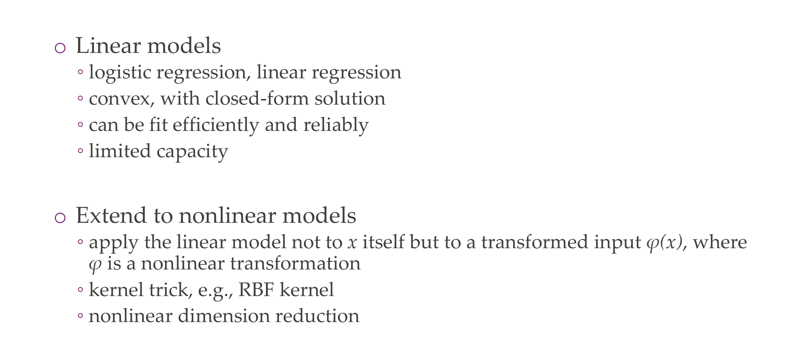
Here we are saying that at the end we have just have a linear function \(C\) “the linear model” ie.
\[ C(\sigma(B\sigma(A\textbf{x}))) \]
to a transformed input \(\varphi(x\textbf{x})\) = \(\sigma(B\sigma(A\textbf{x}))\)
5 How to get w? gradiend-based learning
- Due to nonlinearity our loss function would be nonconvex
- We use then SGD
- No guarantee of convergence, and sensitive to initialization of the parameters
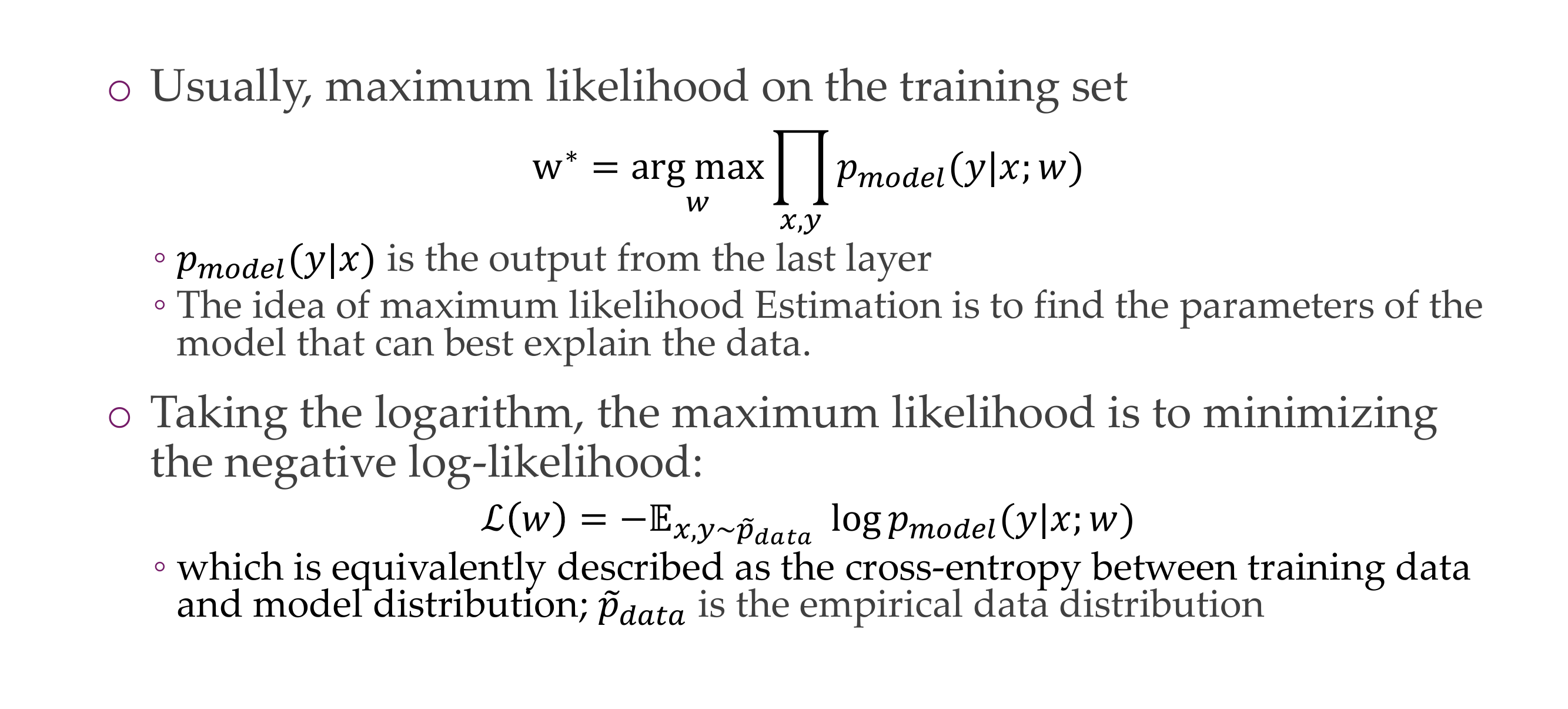
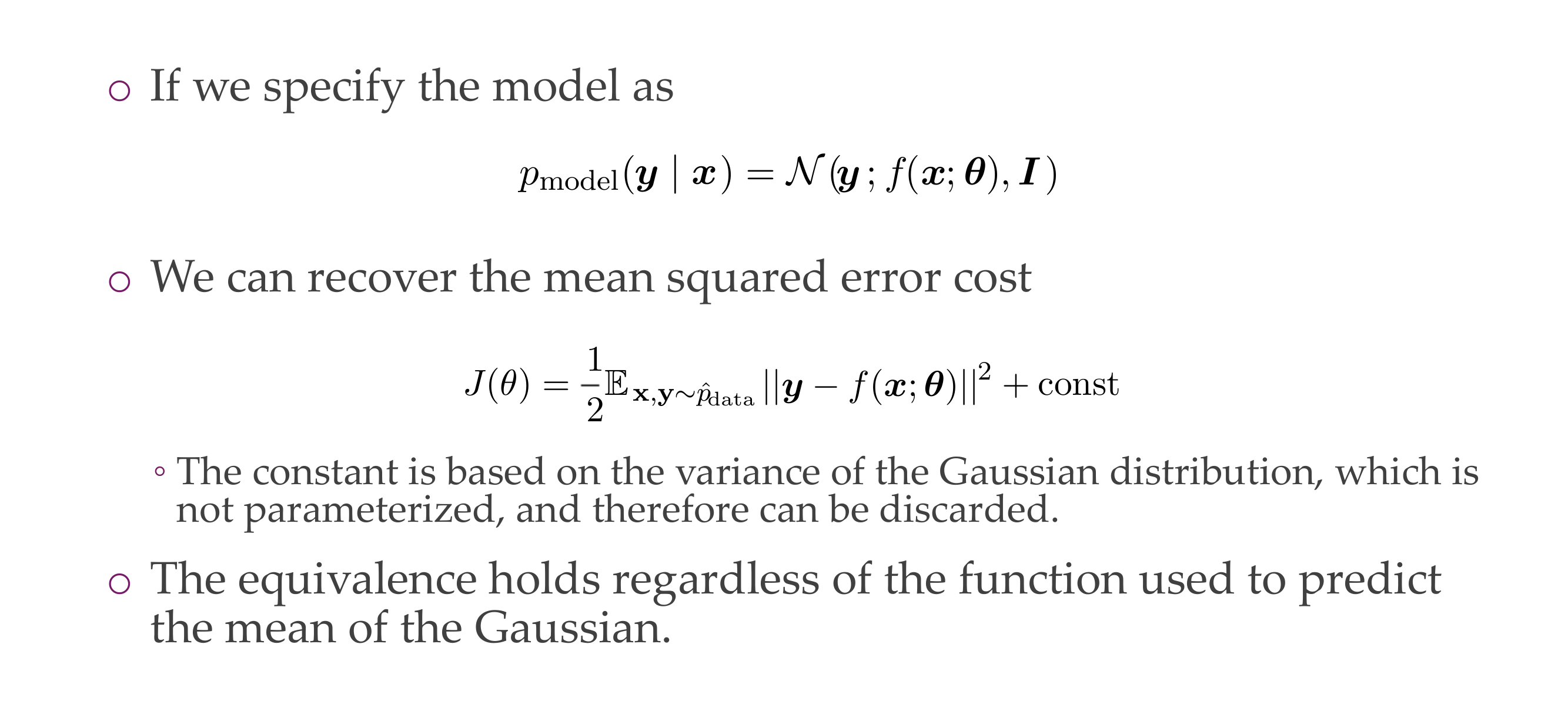
6 Cost Function
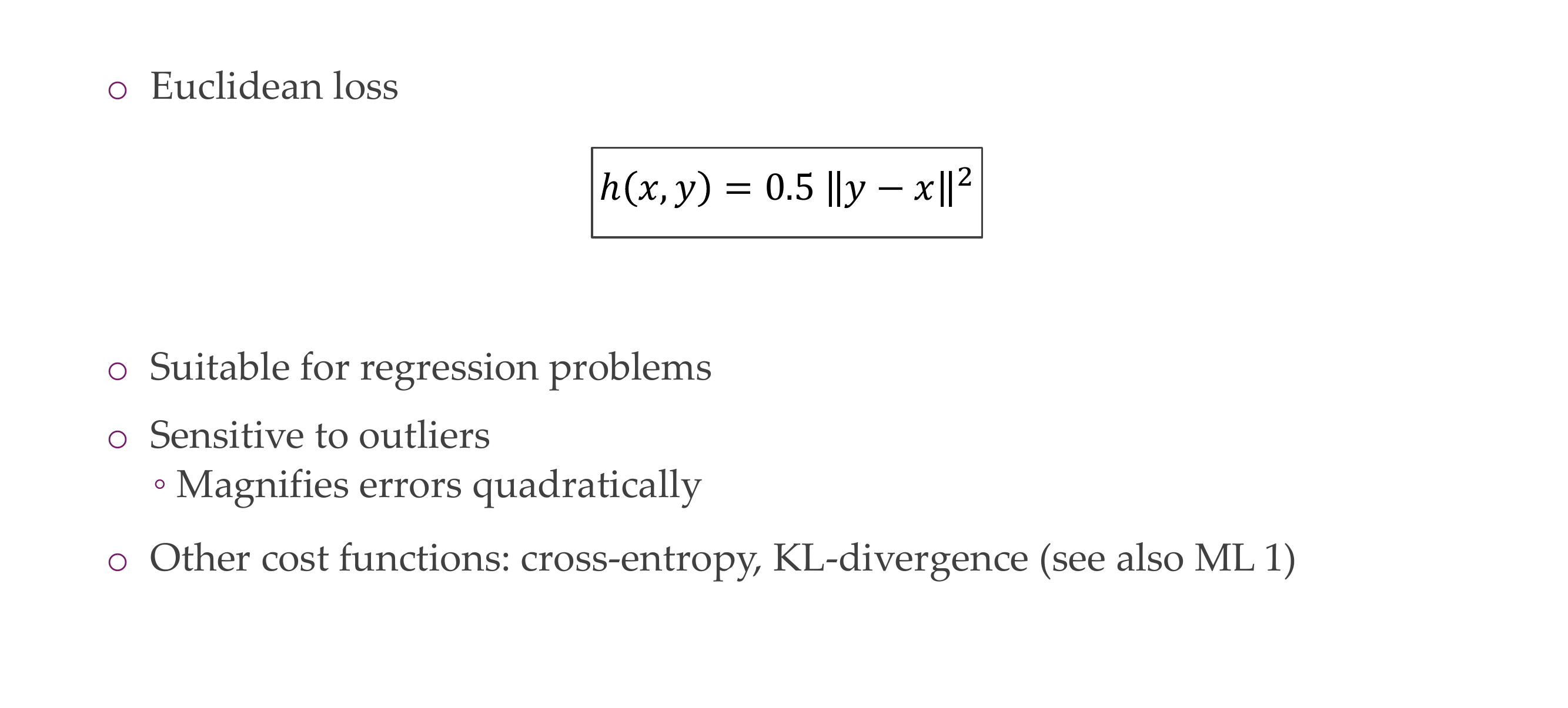
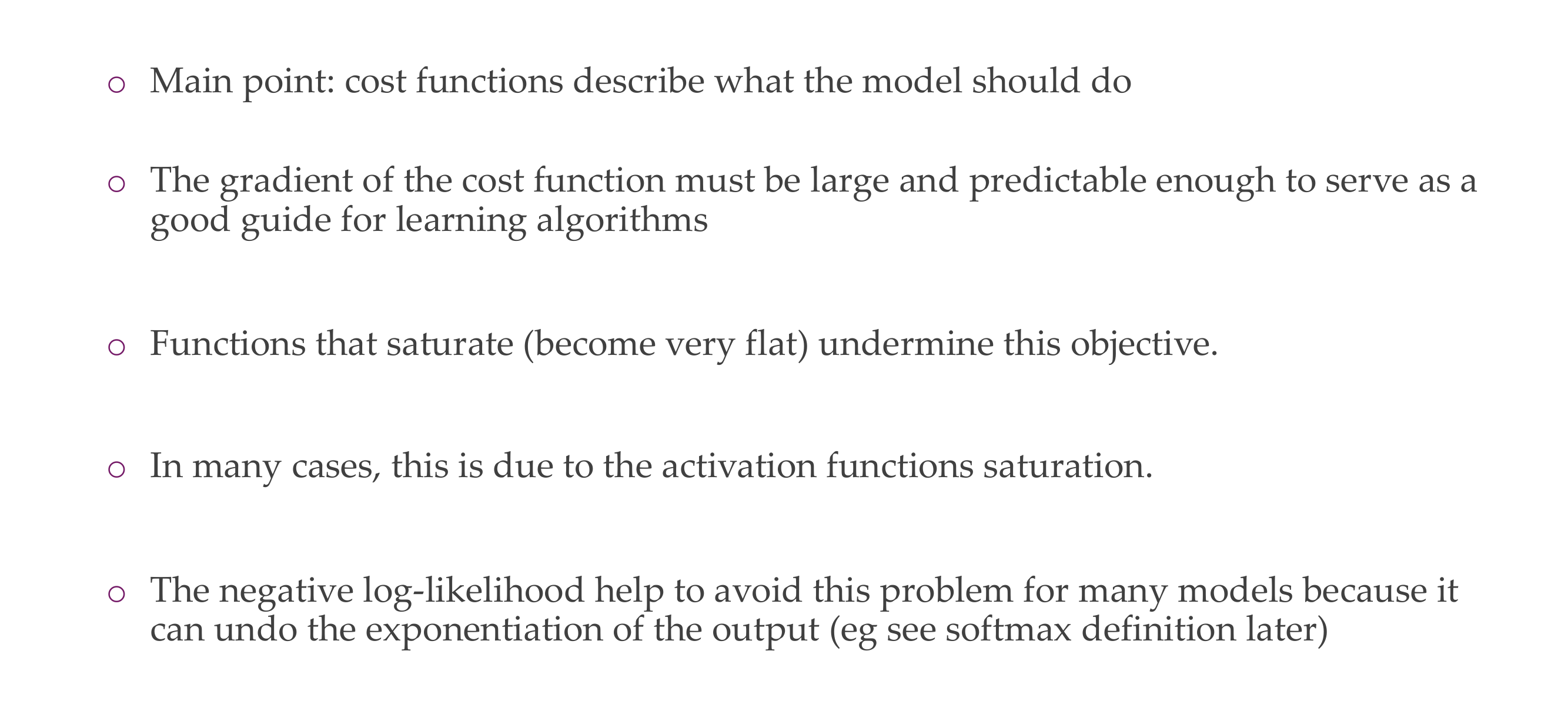
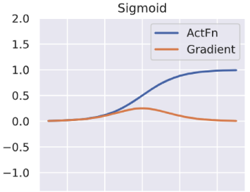
Here saturated means that the function becomes very flat so then the gradient of this is very minimal so then we cannot compute optimize because all the derivatives would look like very similar
7 Activation Functions
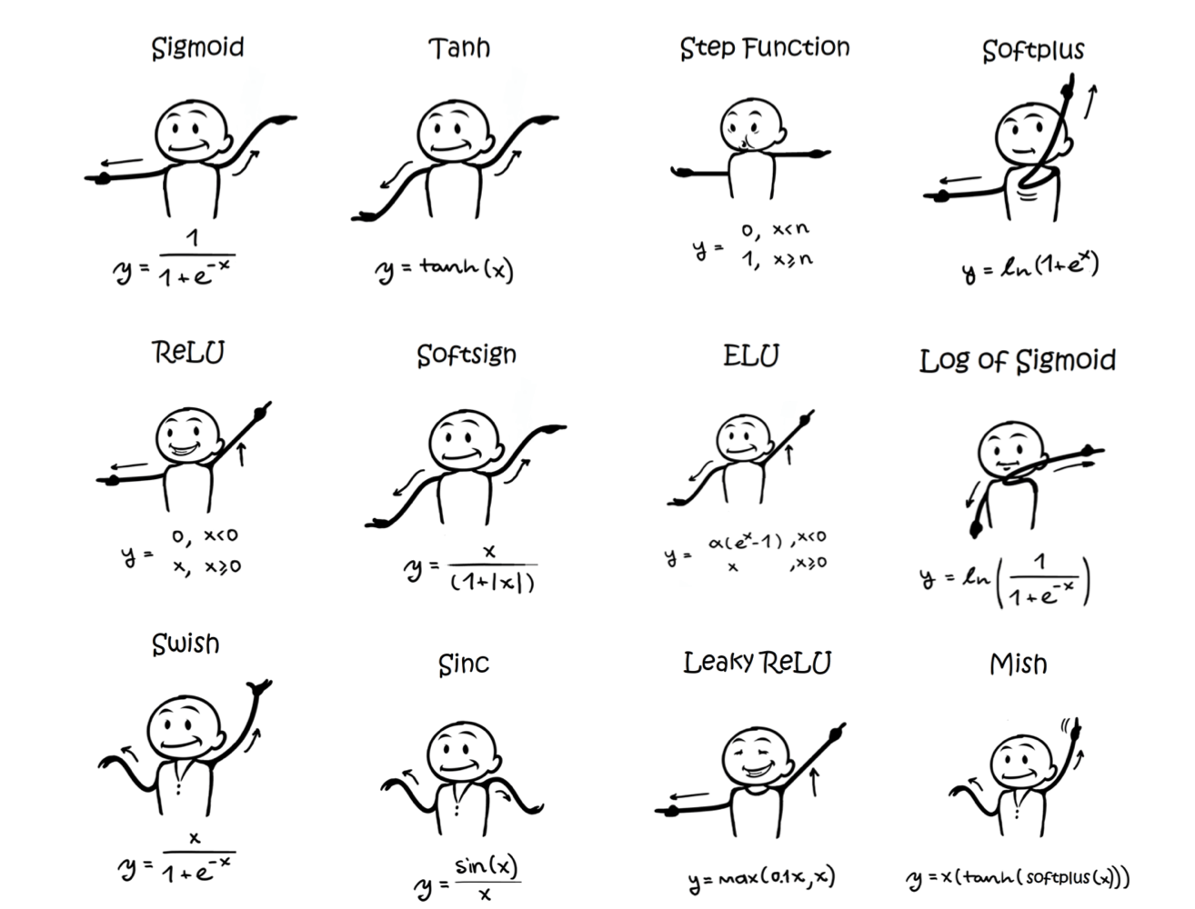
- Defined how the weighted sum of the input is transformed into an output from a node or nodes in a layer of the network.
- If output range limited, then called a “squashing function.”
- The choice of activation function has a large impact on the capability and performance of the neural network.
- Different activation functions may be combined, but rare
- All hidden layers typically use the same activation function
- Need to be differentiable at most points
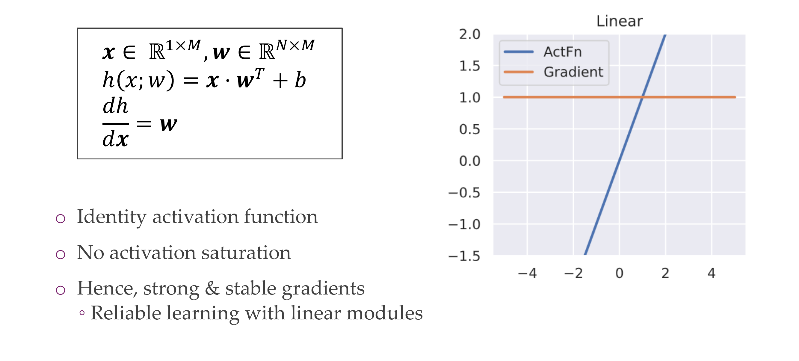
8 Linear Units/ “Fully connected layer”
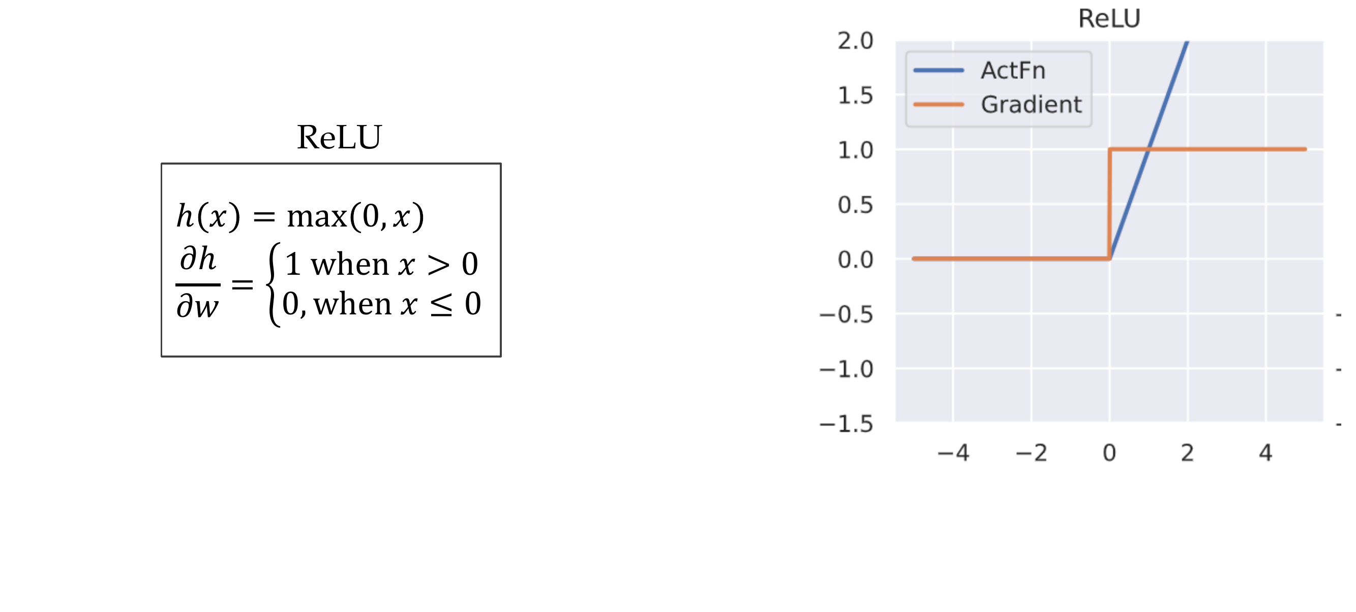
9 Advantages of ReLU
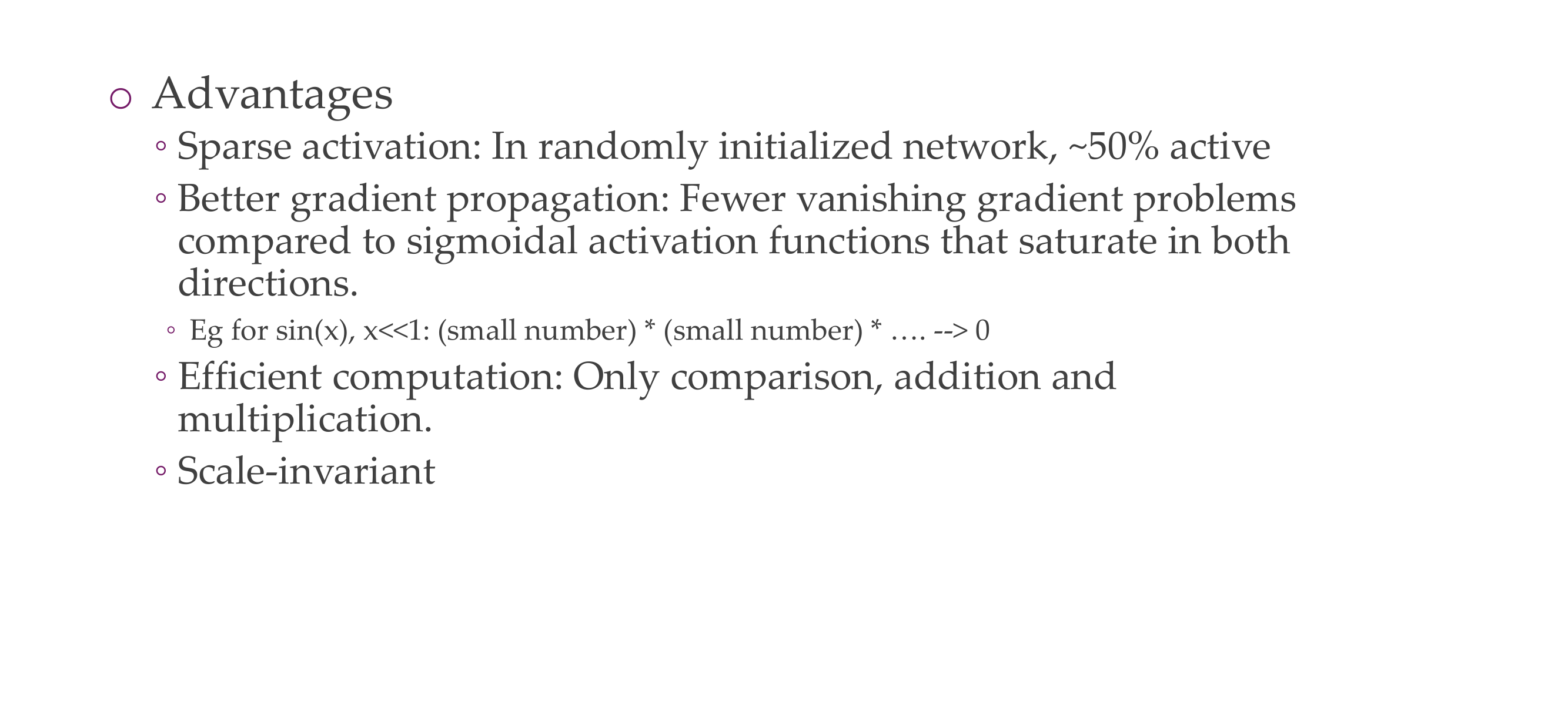
ReLu is better for propagation because if i.e take a sin as activation function when we derive close to zero the gradient would be very small, we keep doing this over multiple layers and essentially multiplying small times smalls at the end the result would be close to \(0\).
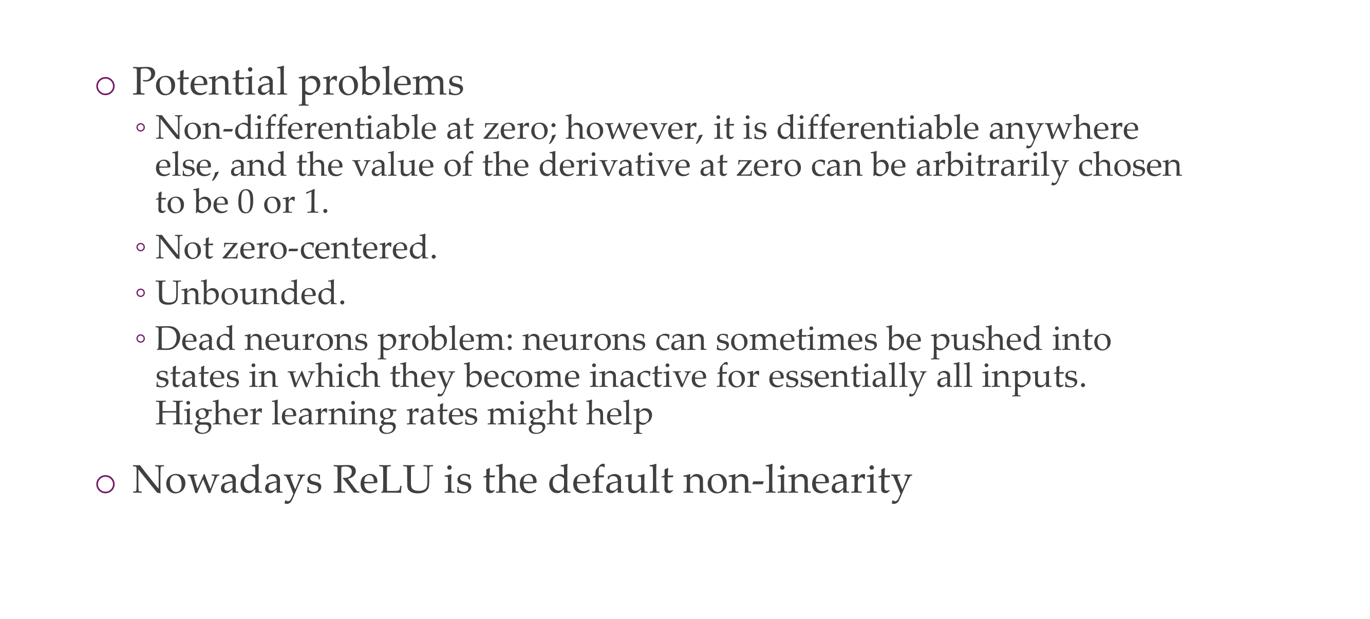
10 Disadvantages of ReLU
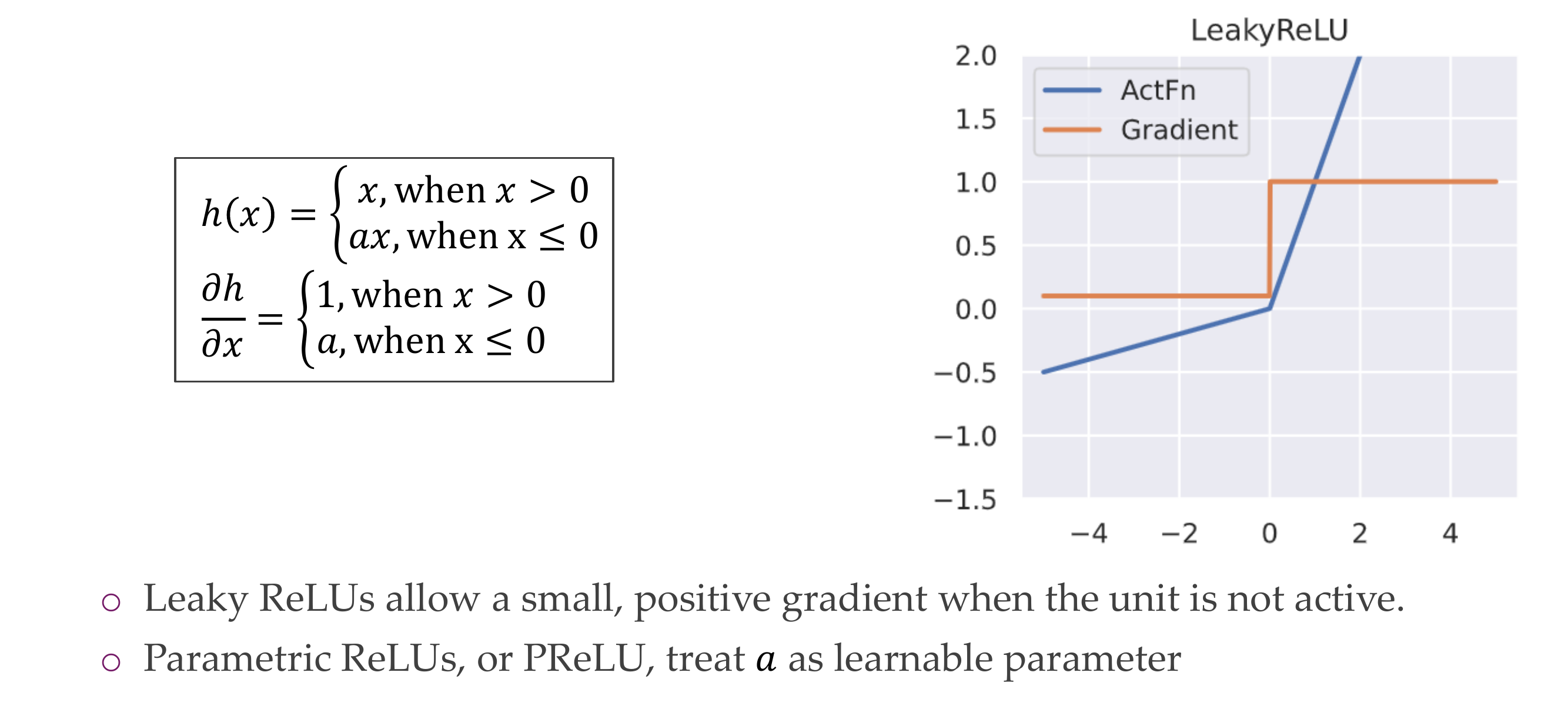
11 Leaky ReLU
12 Exponential Linear Unit (ELU)
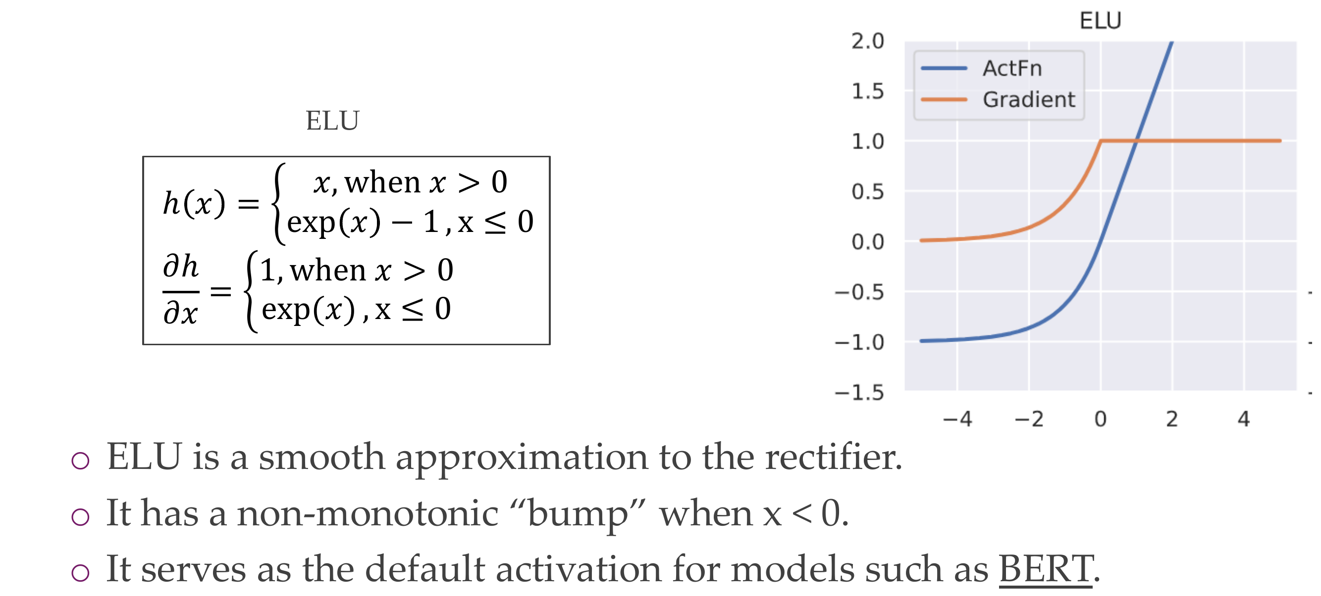
Used in Language models like BERT
13 Gaussian Error Linear Unit
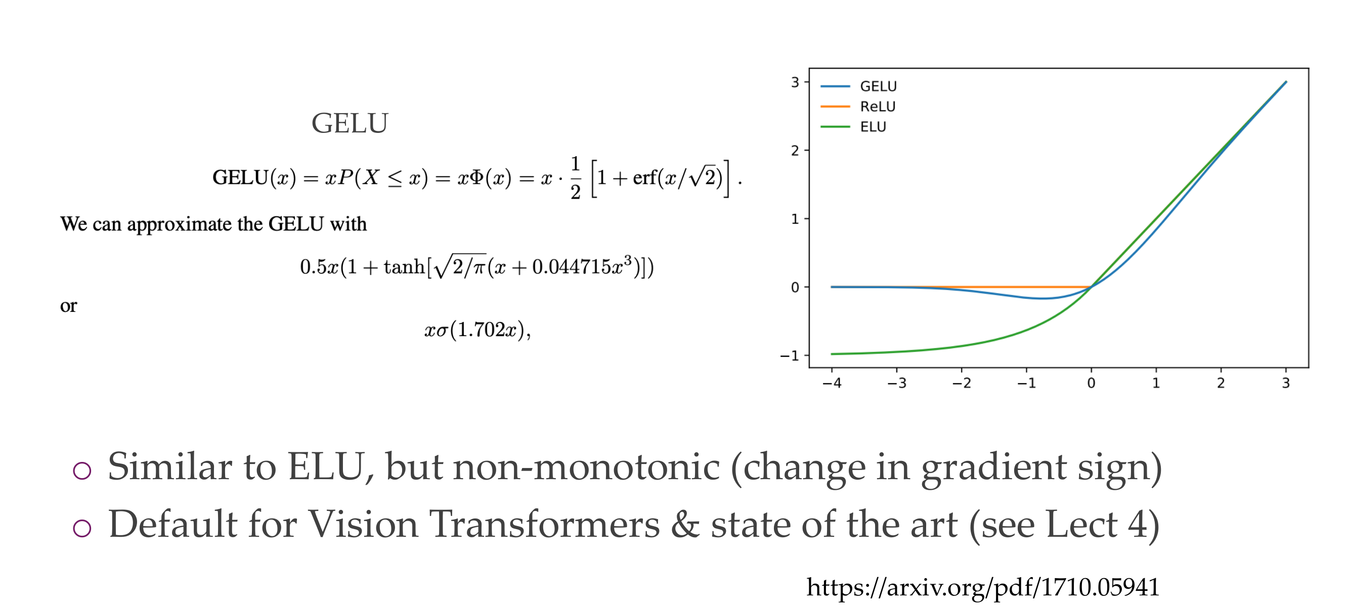
We are not bounded by the computation power but by memory to be loaded in the computation units of the GPUs on Snellius
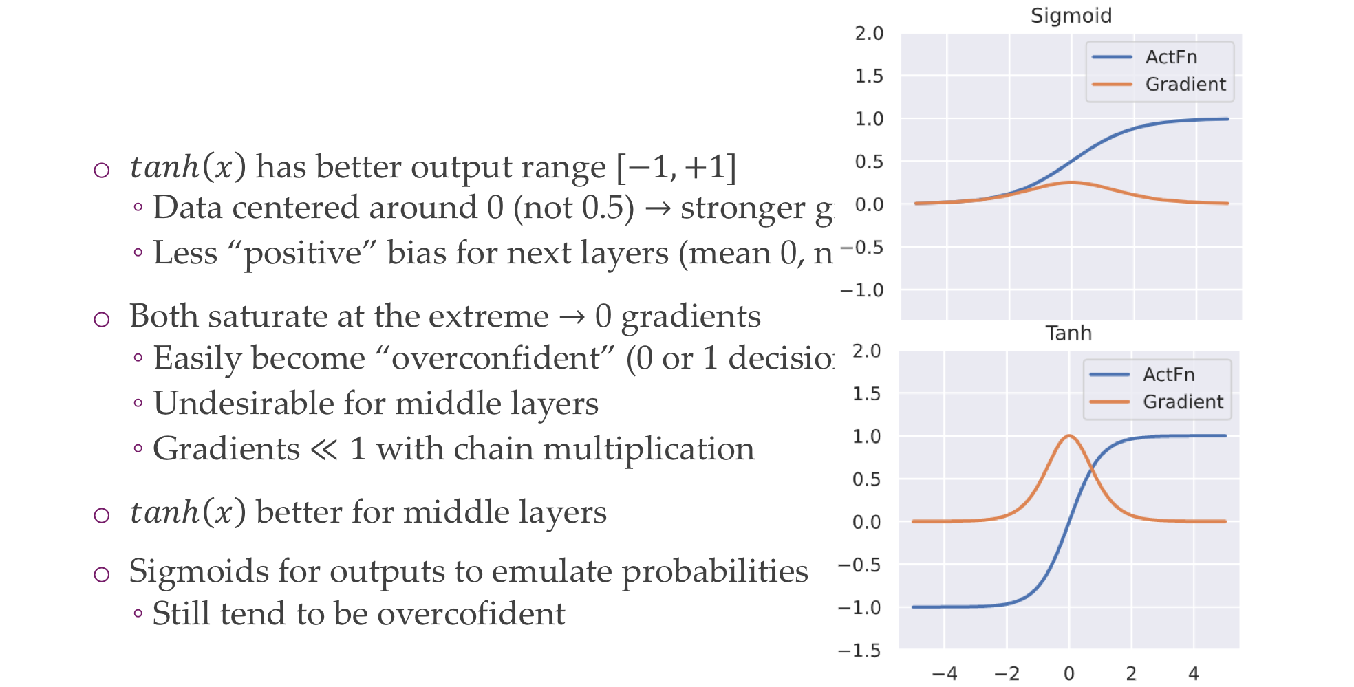
14 Sigmoid and Tanh

15 Softmax
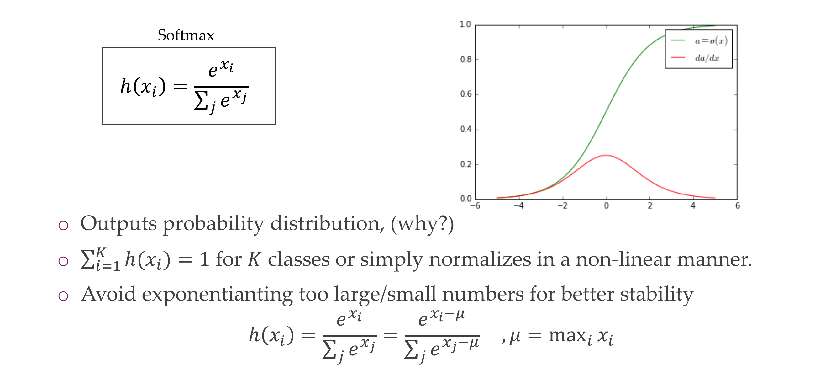
It outputs a probability distribution because it depends on the denominator which means all the variables would be taken into account. For instance this can be the last activation function to output probabilities of predicting a cat, a dog, a bird and so on.
If we now introduce a term \(\tau\) in Softmax (by dividing the \(e^{\frac{x_i}{\tau}}\) in the numerator and denominator) then we have the following:
If τ is introduced, it can be used to control the temperature or the “sharpness” of the softmax distribution.
When τ is set to a value greater than 1, it has the effect of “softening” the probabilities, making the distribution more uniform. In other words, it makes the probability of all categories more similar to each other. This can be useful in scenarios where you want to explore a wider range of possibilities or reduce the impact of extreme values in the input vector.
Conversely, when τ is set to a value less than 1, it has the effect of “sharpening” the probabilities, making the distribution more peaky, and emphasizing the largest values in the input vector. This can be useful when you want to make more distinct predictions and reduce uncertainty.
16 How to Choose and Activation Function
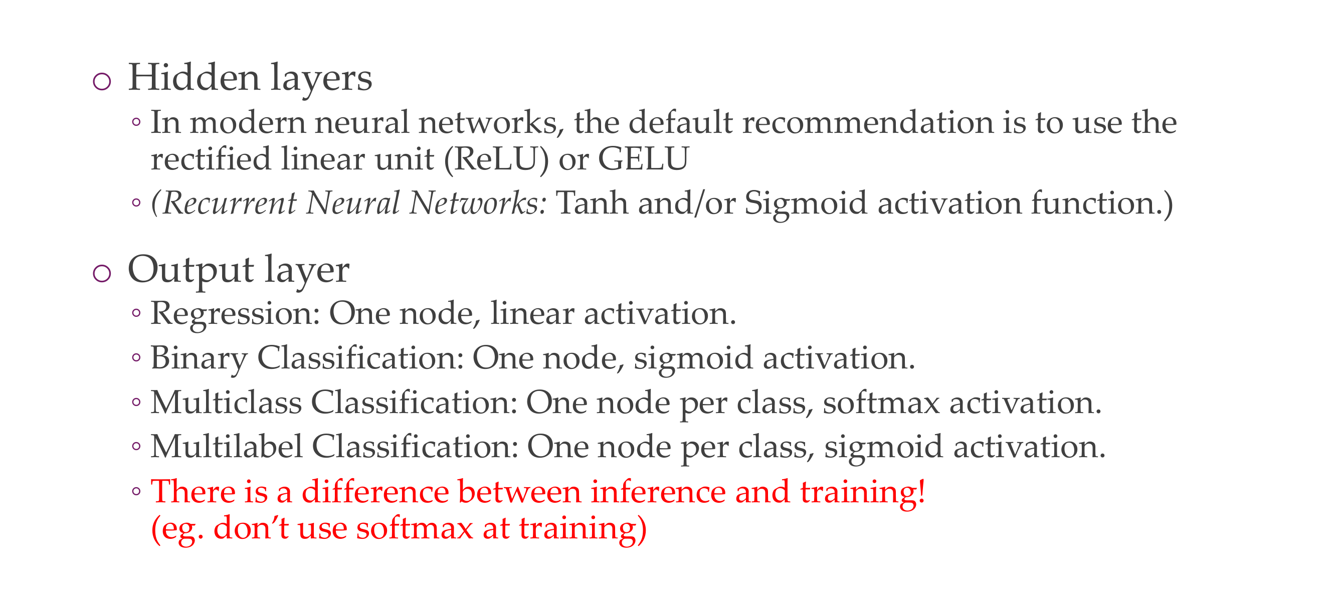
Here inference is testing or predicting
16.1 Difference between Multiclass classification vs Multilabel calssification
Multiclass Classification:
- In multiclass classification, the task is to assign an input data point to one and only one class or category from a set of multiple mutually exclusive classes.
- Each data point belongs to exactly one class, and the goal is to determine which class that data point most likely belongs to.
- Examples of multiclass classification problems:
- Handwritten digit recognition: Given an image of a handwritten digit (0-9), determine which digit it represents.
- Species classification: Given a photo of an animal, classify it into one of several species (e.g., dog, cat, bird, etc.).
Example: Suppose you have a multiclass classification problem where you want to classify fruits into three categories: apples, oranges, and bananas. If you input an image of an apple, the model should predict that it belongs to the “apples” class.
Multilabel Classification:
- In multilabel classification, each data point can be associated with one or more classes or labels. It’s not limited to assigning a single class per data point.
- This is used when a data point can have multiple attributes or characteristics simultaneously, and you want to predict all relevant labels.
- Examples of multilabel classification problems:
- Document categorization: Tagging a document with multiple topics or subjects that are present in it.
- Image tagging: Assigning tags to an image to describe its content, where an image may contain multiple objects or scenes.
Example: Consider an image tagging problem. You have an image containing a beach scene with a dog and a sunset. In a multilabel classification scenario, the model might predict the following labels: “beach,” “dog,” and “sunset,” because all three labels are relevant to the image.
In a multiclass classification problem, the softmax function is commonly used to convert the raw output scores of a model into a probability distribution over multiple classes. This probability distribution allows you to determine the likelihood of each class for a given input data point. Here’s how you use the softmax function in a multiclass classification problem:
- Model Output:
- After training your multiclass classification model, you will typically have a final layer in your neural network or a scoring function that produces raw scores (logits) for each class. These scores are not yet probabilities but represent the model’s confidence in each class.
- Let’s say you have N classes, and the model’s output for a particular input is a vector of raw scores \(z\) with N elements, one for each class.
- Apply Softmax Function:
- To convert the raw scores into probabilities, apply the softmax function to the \(z\) vector. The softmax function transforms the scores into a probability distribution where the sum of the probabilities for all classes equals 1.
- The softmax function for class \(i\) is given by: \(\text{softmax}(z)_i = \frac{e^{z_i}}{\sum_{j=1}^N e^{z_j}}\)
- Calculate the softmax value for each class \(i\) in the \(z\) vector to obtain a probability distribution.
- Predict the Class:
- The class with the highest probability in the softmax distribution is typically chosen as the predicted class for the input data point. In other words, the class with the highest \(\text{softmax}(z)_i\) value is the model’s prediction for that input.
Here’s a step-by-step example of using softmax for multiclass classification:
Suppose you have a multiclass classification problem with three classes: “cat,” “dog,” and “bird.” After processing an input image, your model produces the following raw scores:
\(z = [2.1, 0.9, 1.5]\)
- Apply the softmax function:
- Calculate the softmax values for each class:
\(\text{softmax}(z)_1 = \frac{e^{2.1}}{e^{2.1} + e^{0.9} + e^{1.5}}\)
\(\text{softmax}(z)_2 = \frac{e^{0.9}}{e^{2.1} + e^{0.9} + e^{1.5}}\)
\(\text{softmax}(z)_3 = \frac{e^{1.5}}{e^{2.1} + e^{0.9} + e^{1.5}}\)
- Calculate the softmax values for each class:
- Predict the class:
- The class with the highest softmax probability is the predicted class. In this case, if \(\text{softmax}(z)_1\) is the highest probability, the model predicts “cat.”
Using the softmax function in multiclass classification allows you to obtain a probability distribution over classes and select the most likely class as the model’s prediction.
17 Width and Depth
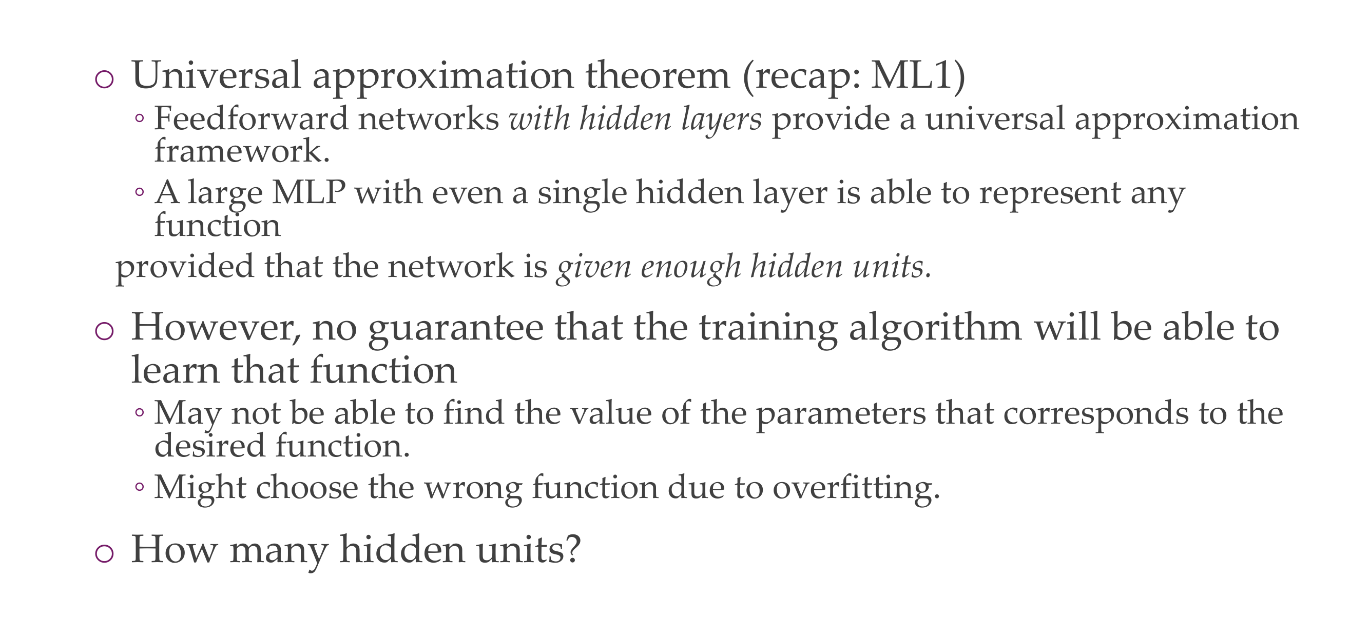
If we have a single big hidden layer (so a lot of parameters) can approximate any functions but in practice this infeasible.
- Width is how many neurons in a single layer
- Depth is the number of layers
This also does not tell you how many hidden units you would need. The theorem just says to approx any function you need infinitely.
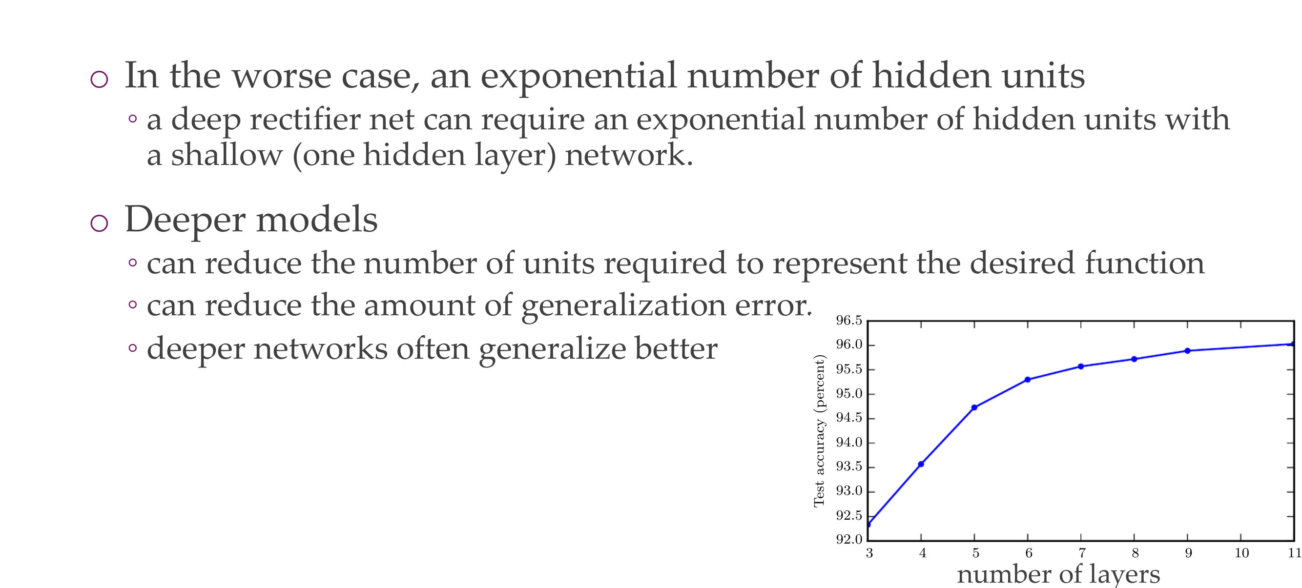
Here we are saying that Deeper models reduce the loss functions (reduce the generalization error) because they generalize better meaning do not overfit. So do not need one single layer with a lot of neurons but instead multiple layers with fewer neurons.
17.1 Convolution Neural Networks vsFully Connected Neural Networks
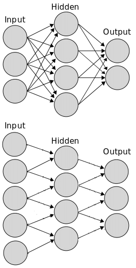
Convolutional needs lees parameters as their inputs are not fully connected to every neuron see pic above
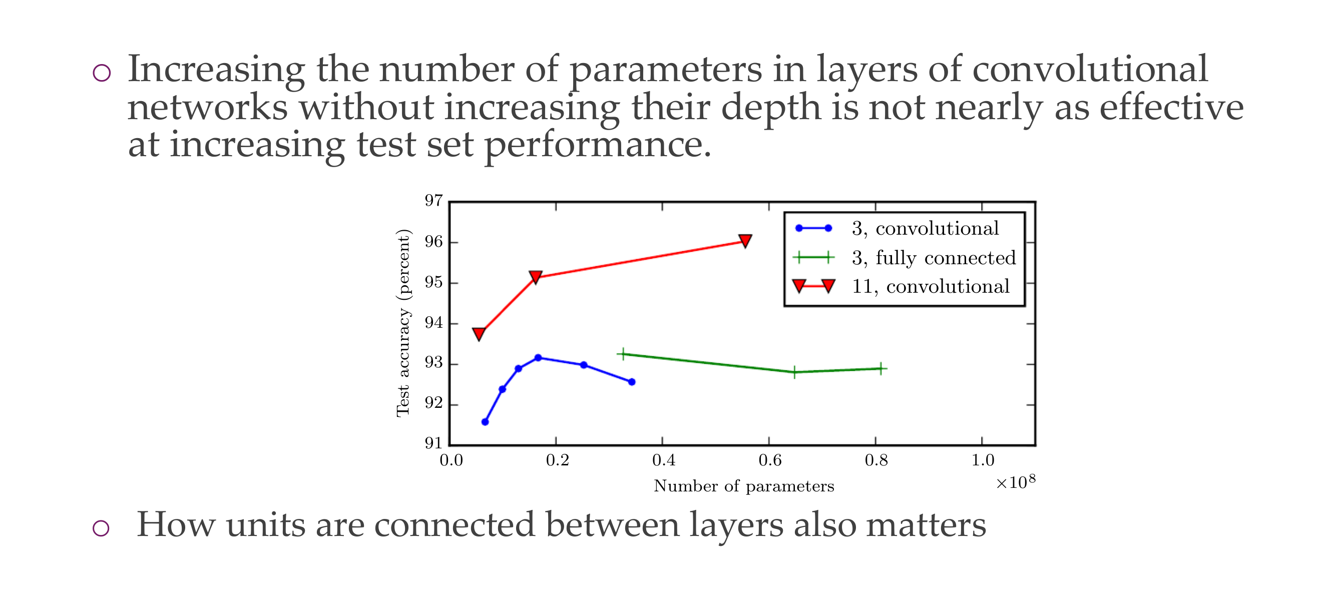
- 3 Convolutional is worse than 11 Convolutional, because the latter is more deeper
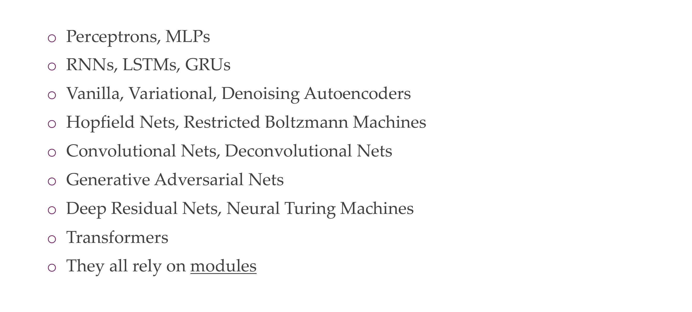
18 Neural Network architectures (jungle)
19 Computational graph
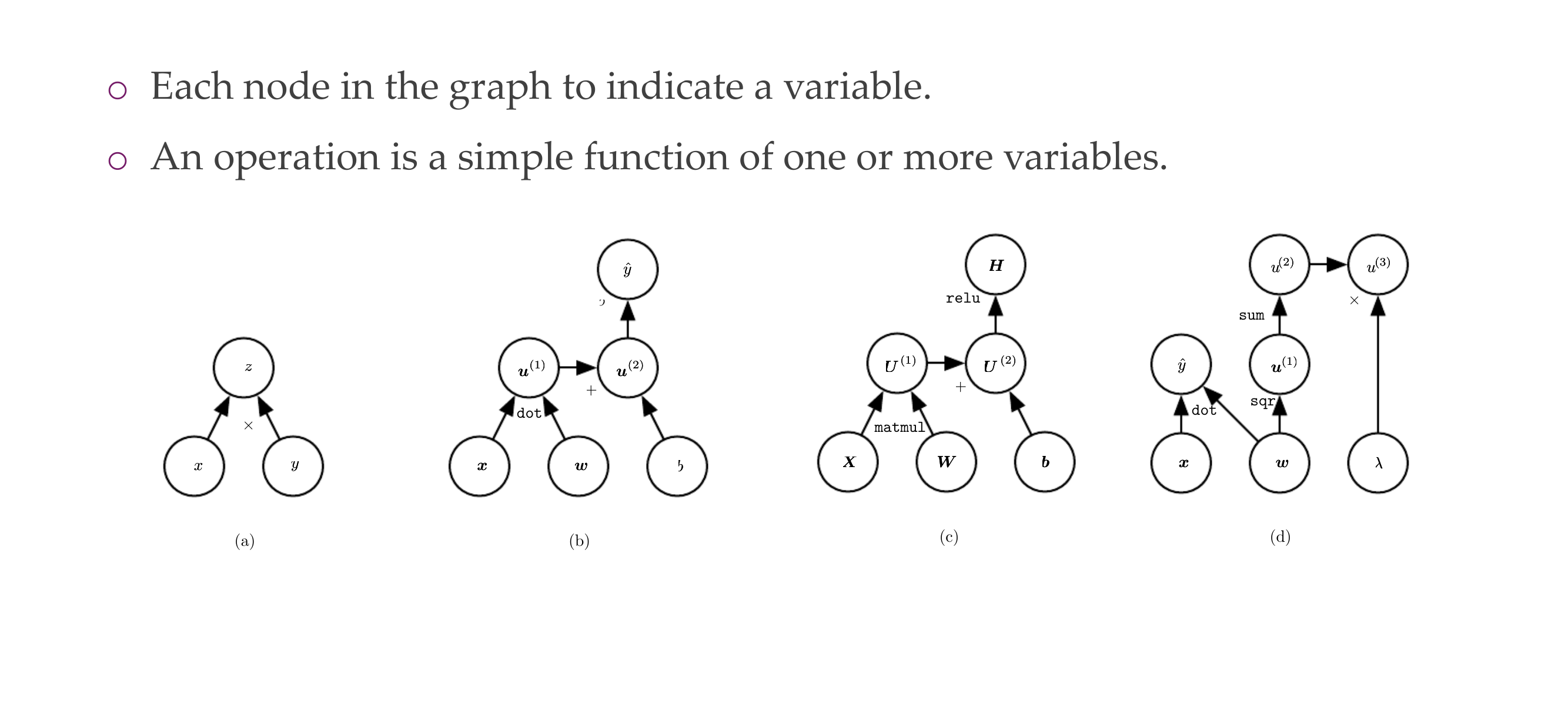
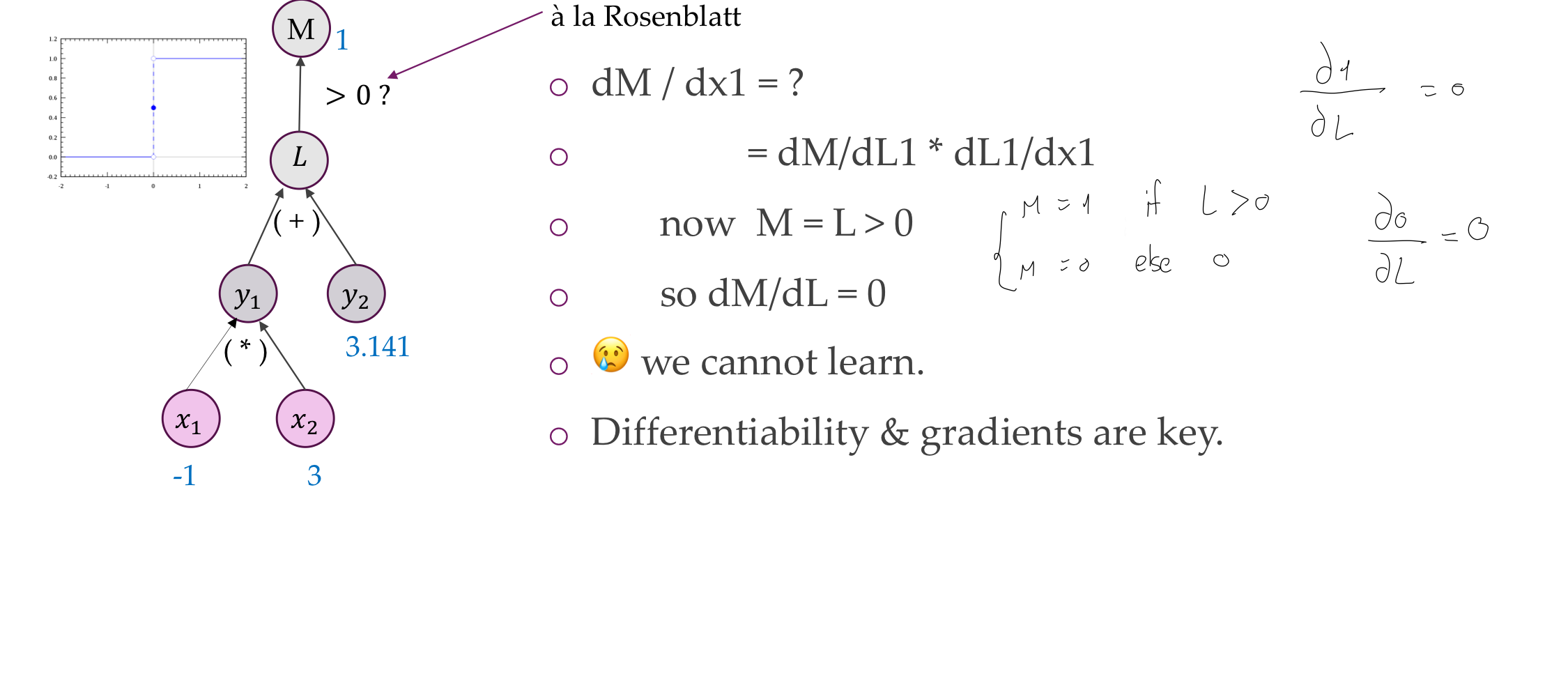
19.1 Example
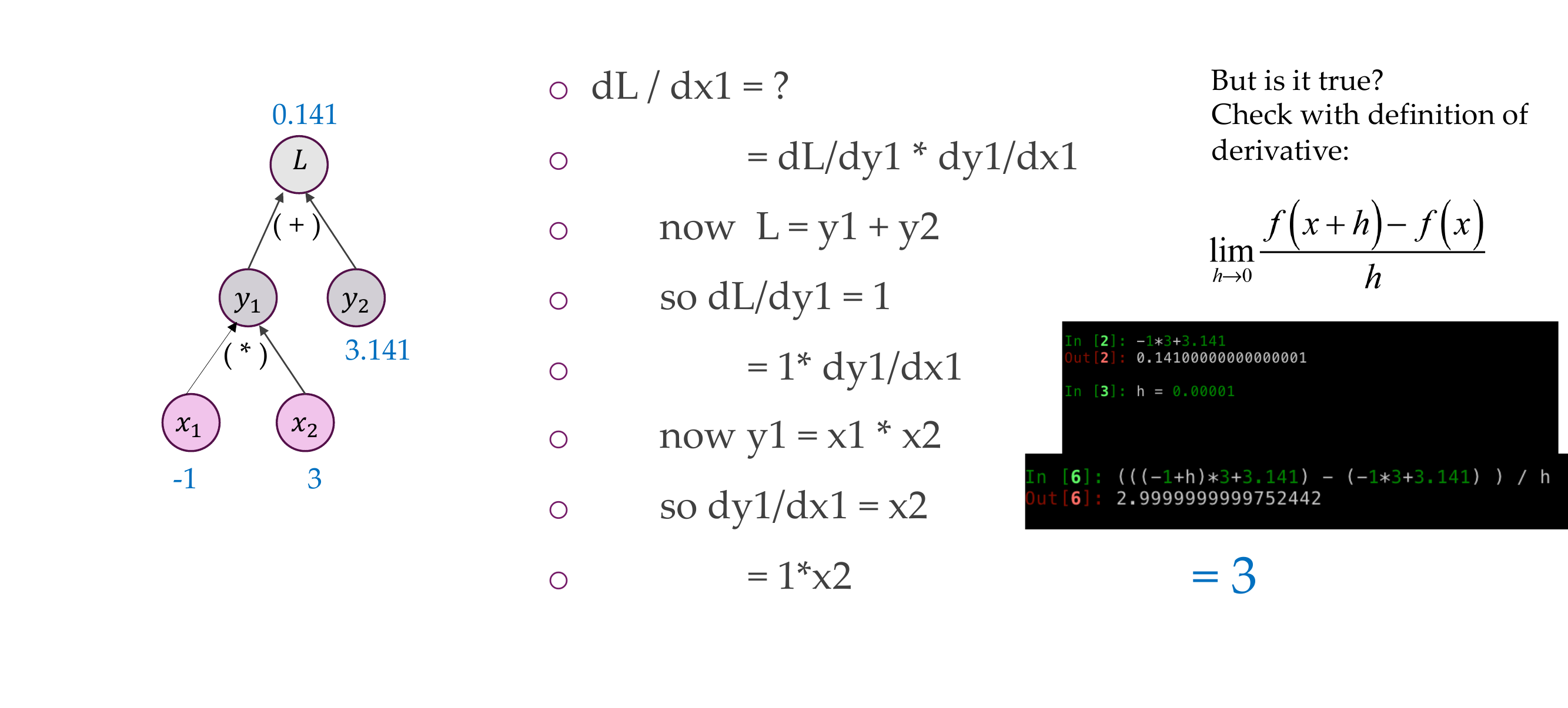
Problem with activation function ReLU
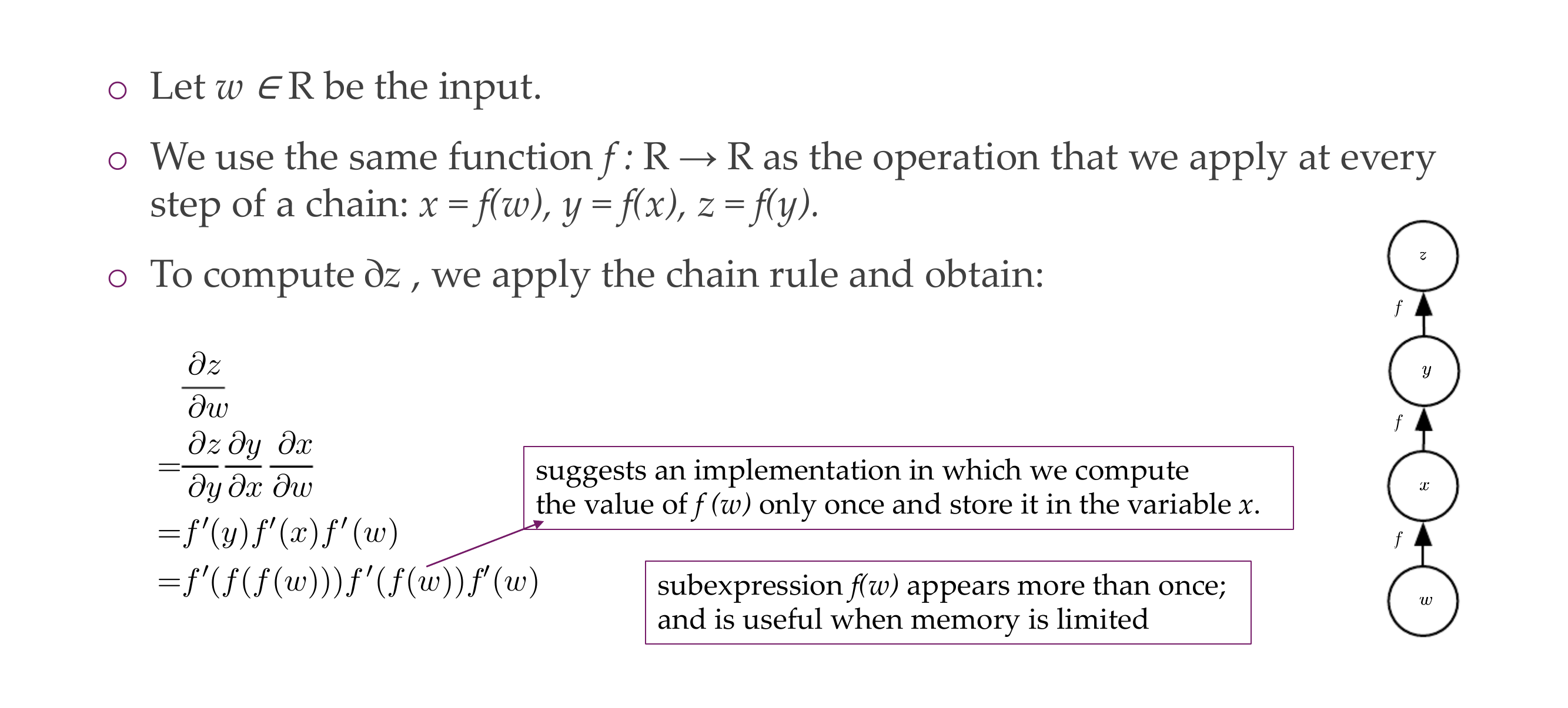
20 Chain Rule of Calculus
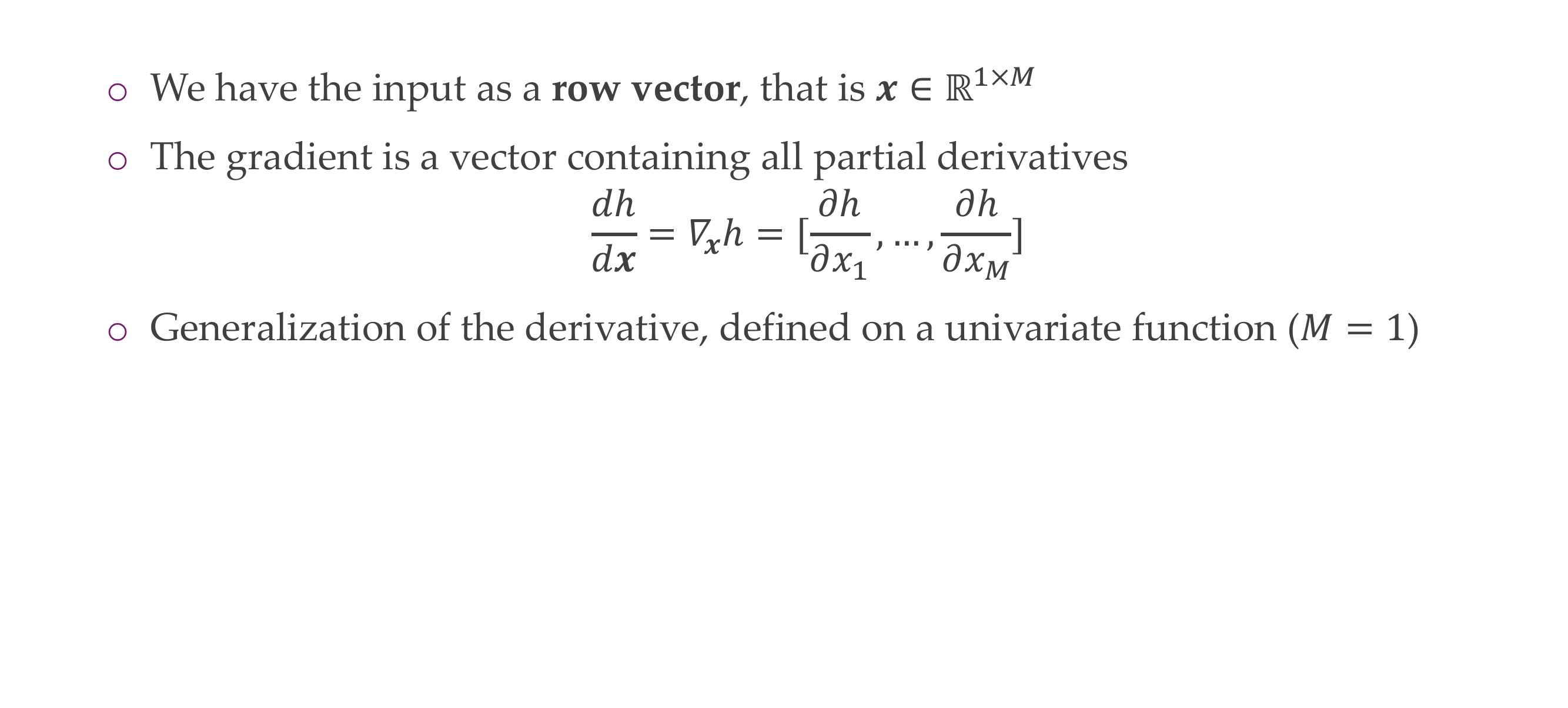
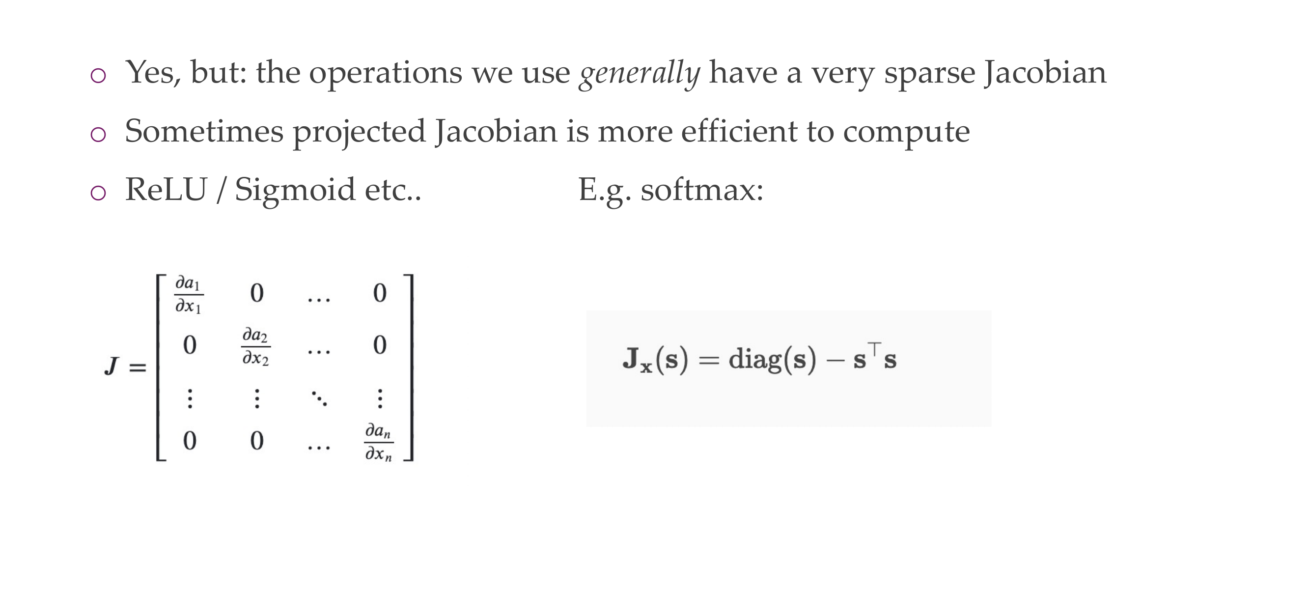
21 The Jacobian
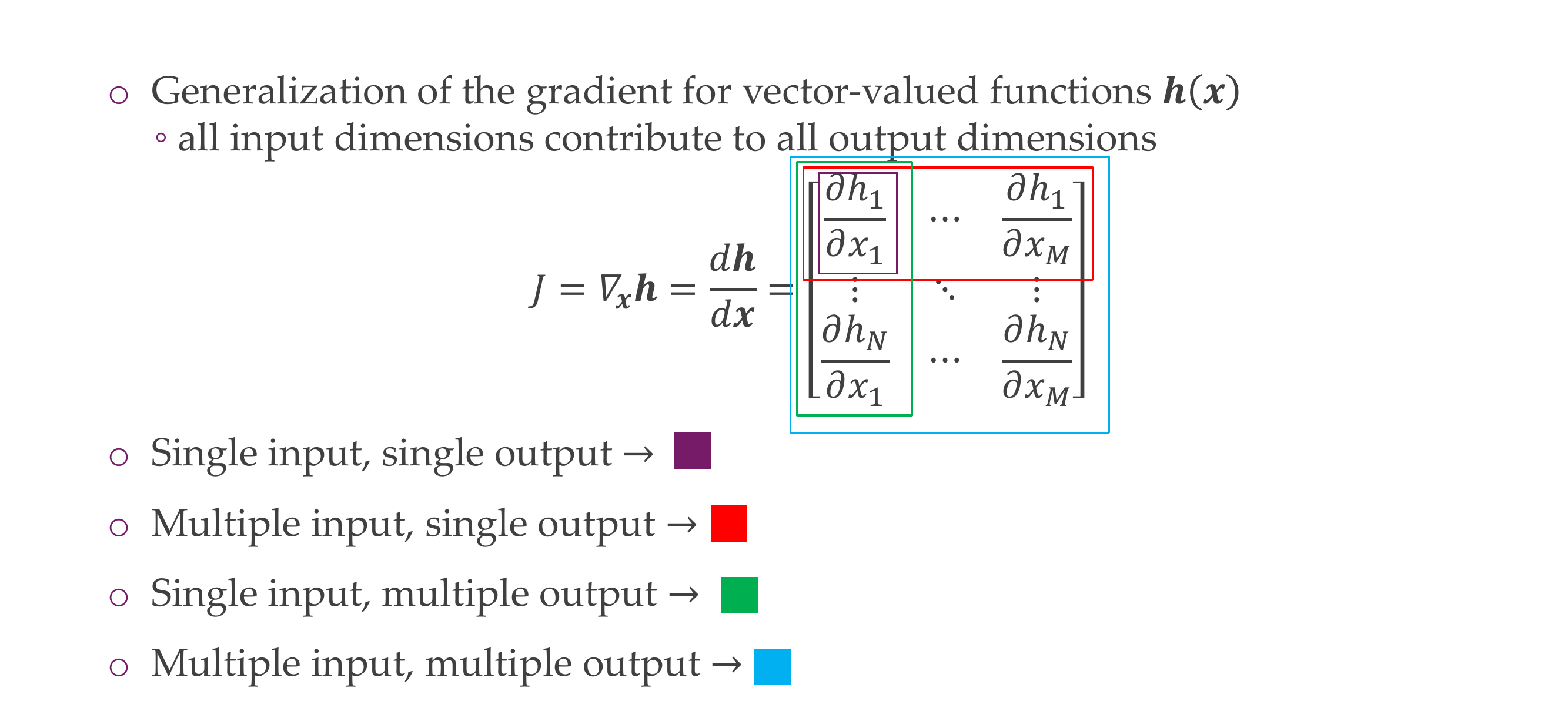
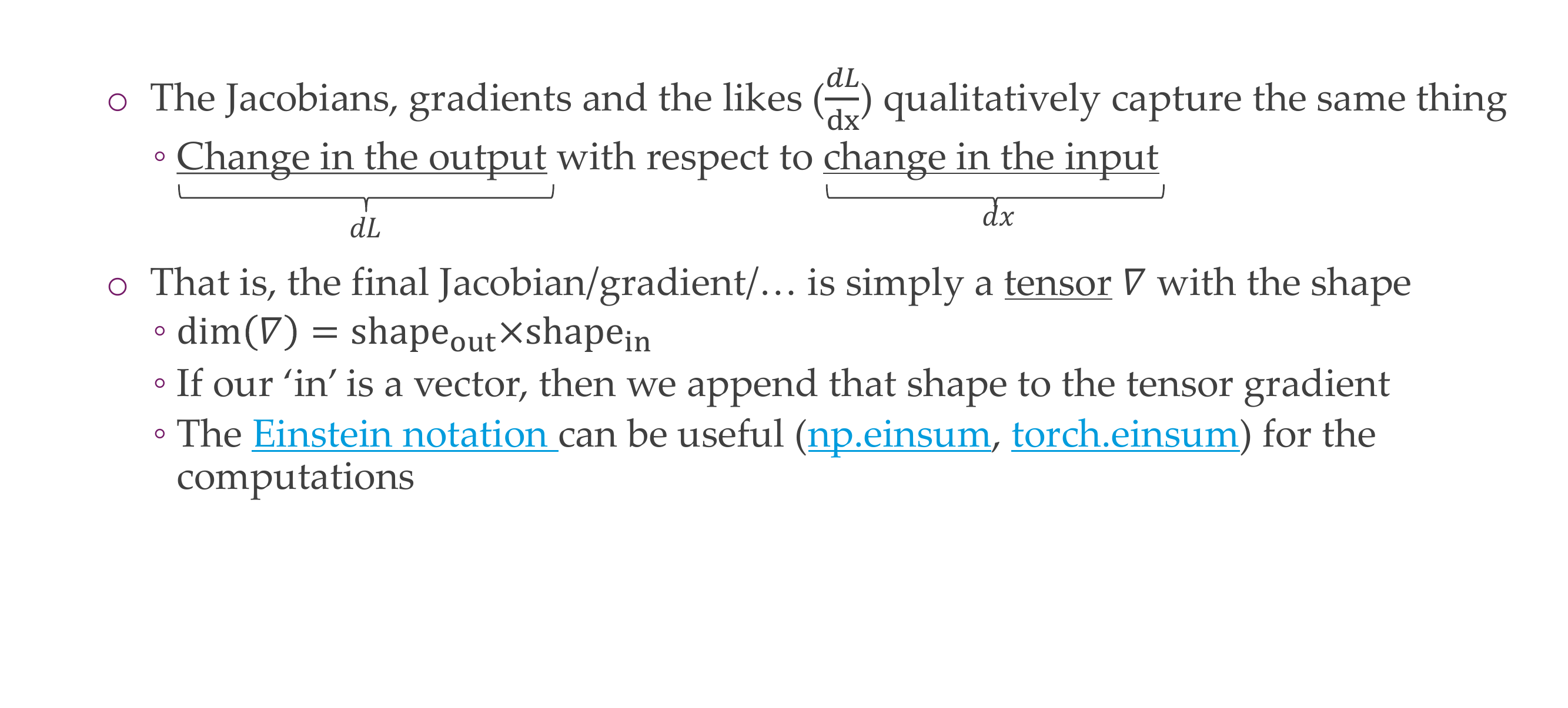
- The Jacobian measures how a change in the input changes the output
- The shape of the Jacobian is ouputs x inputs
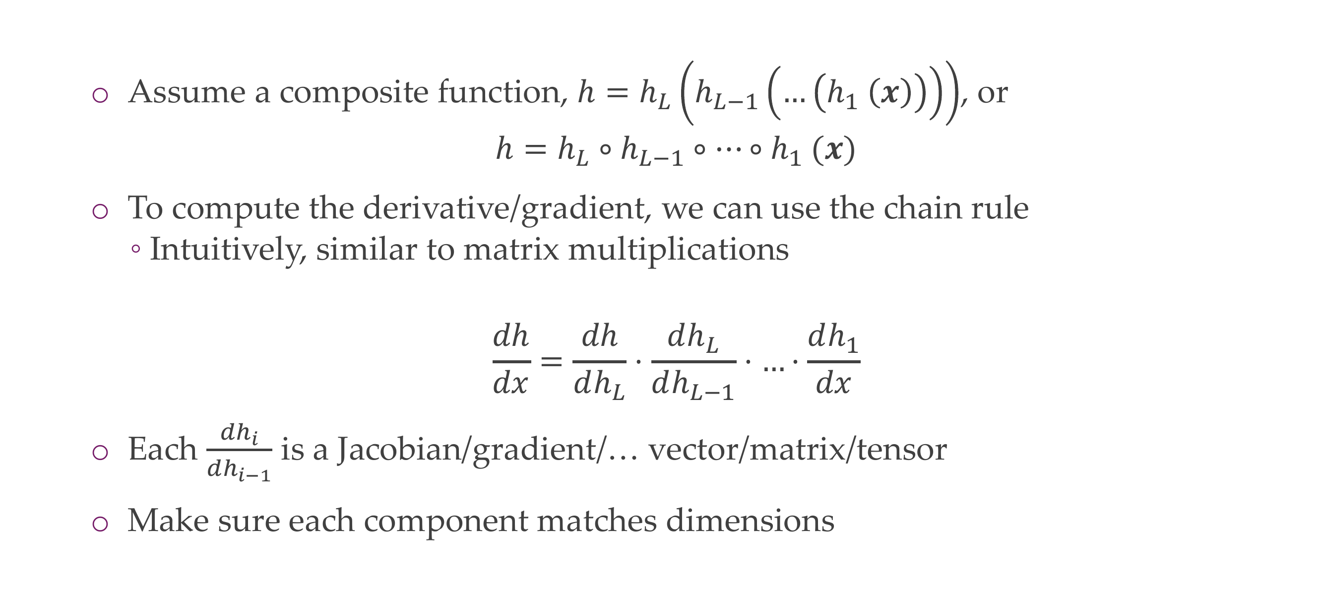
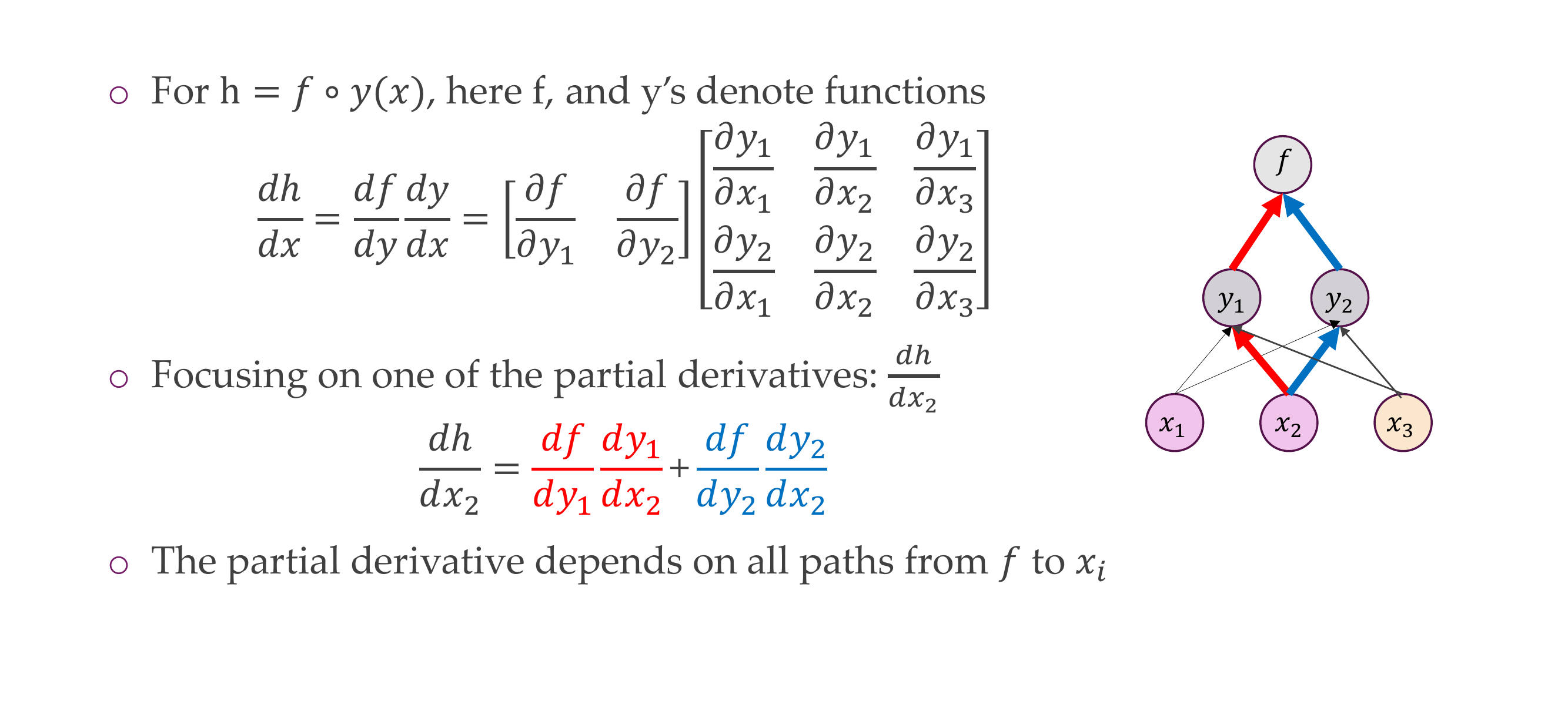
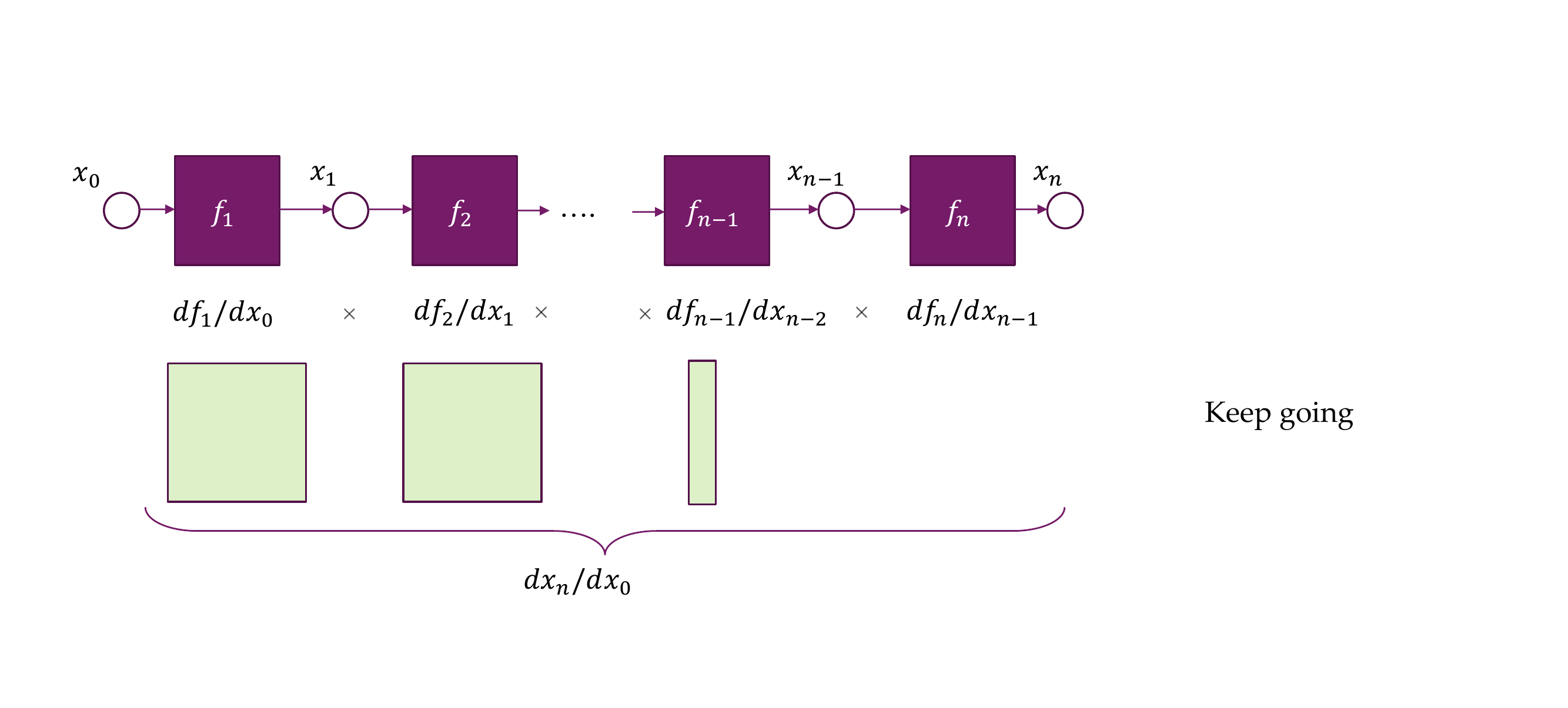
22 Computing gradients in complex functions: Chain rule
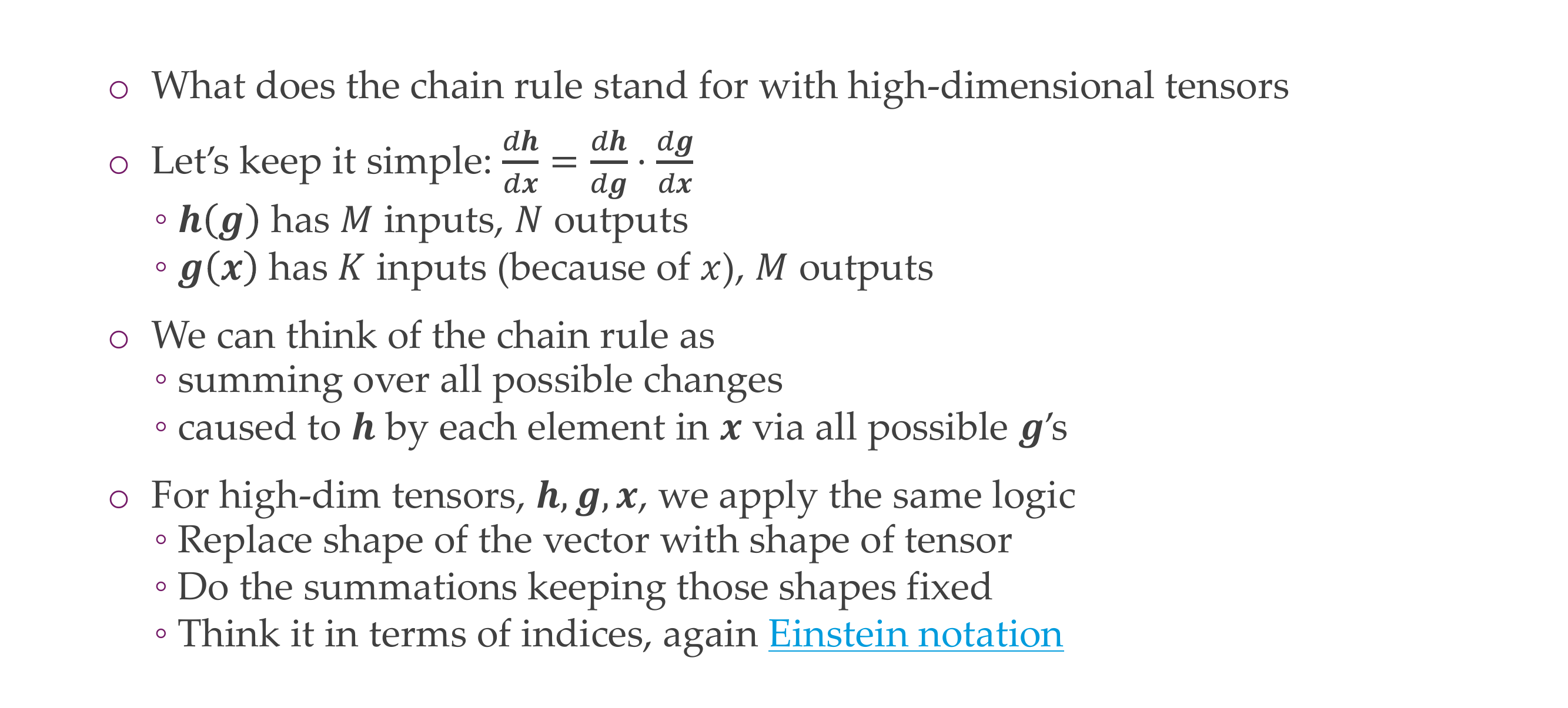
23 Chain rule and tensors, intuitively
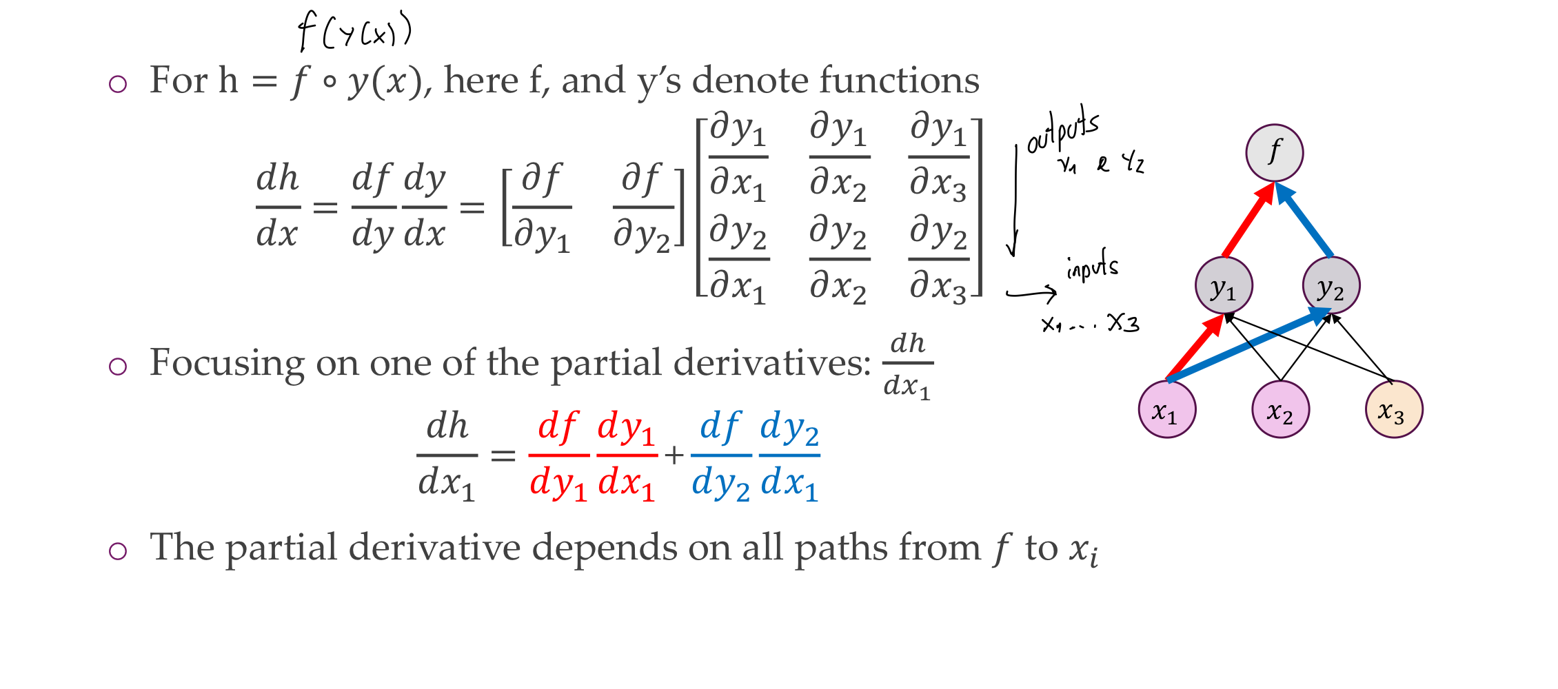
24 Example
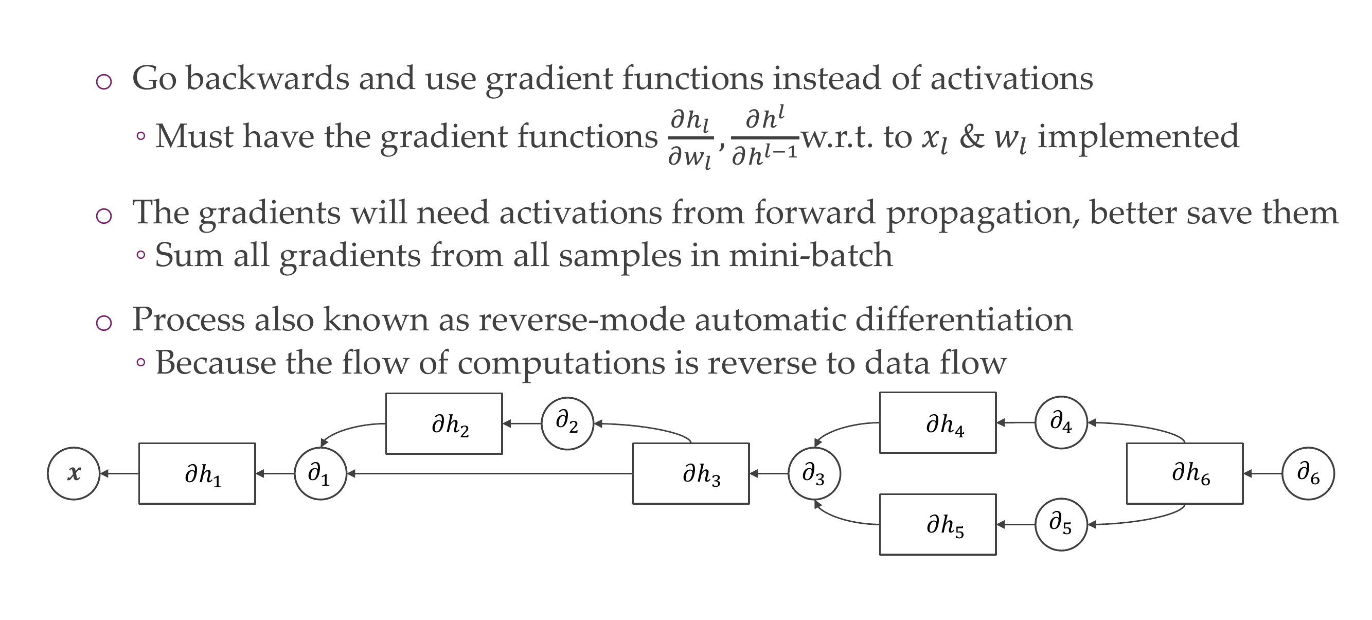
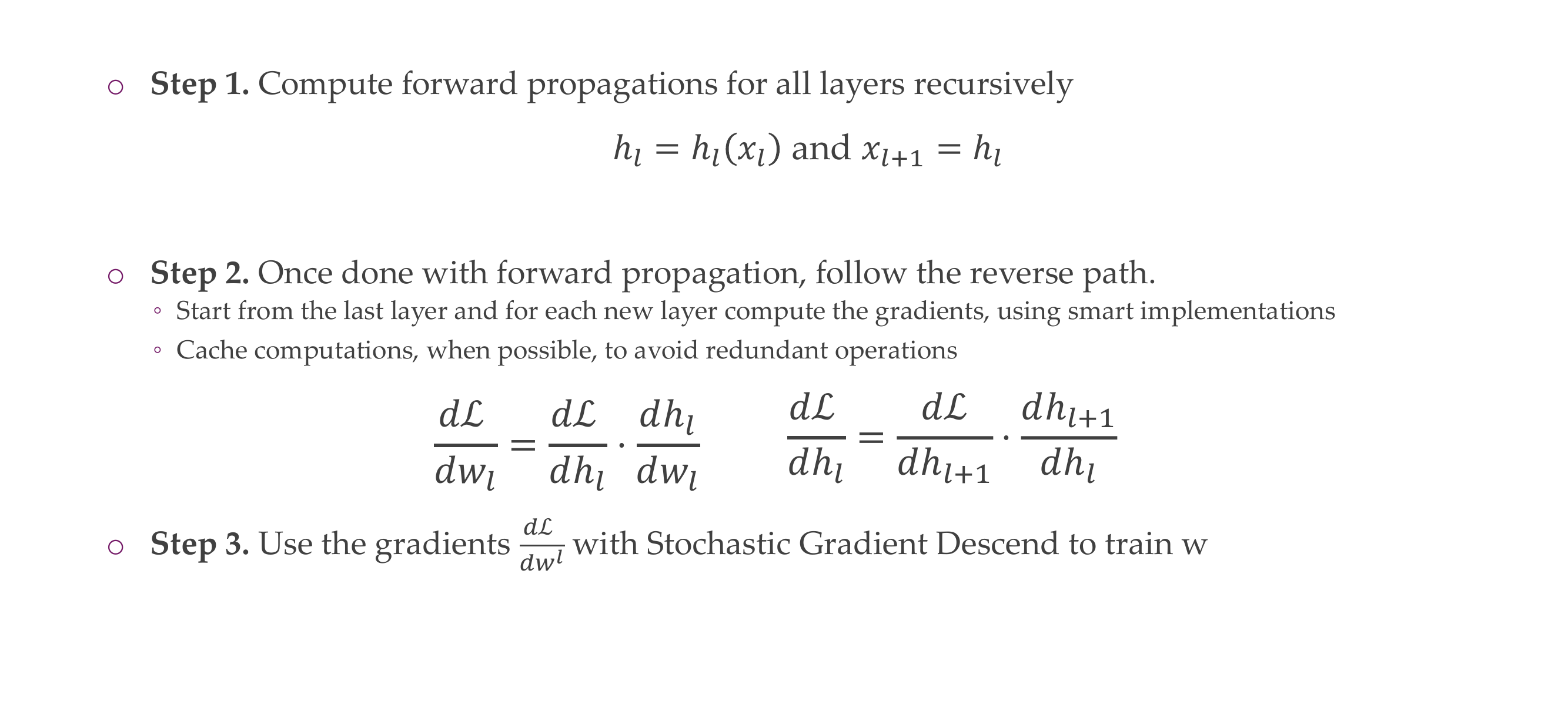
25 Backpropagation Chain Rule
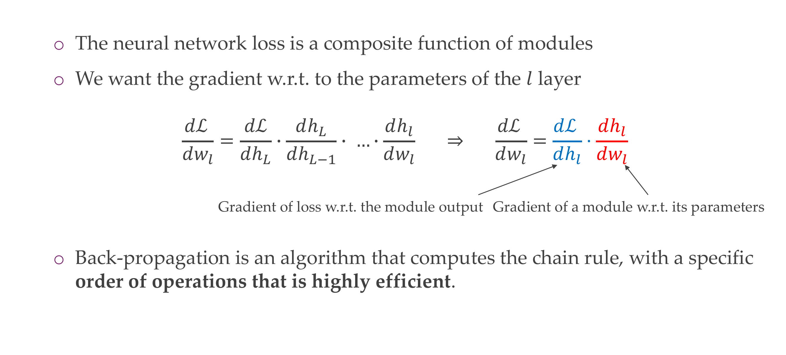
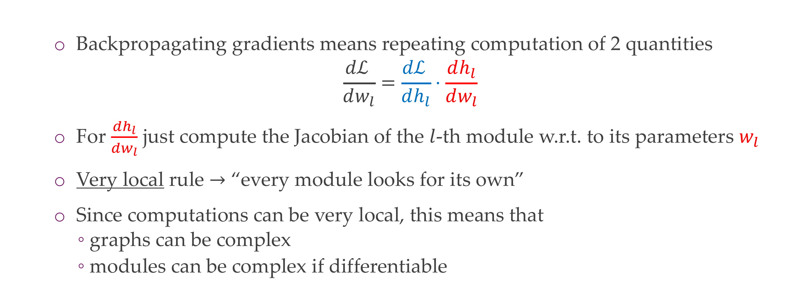
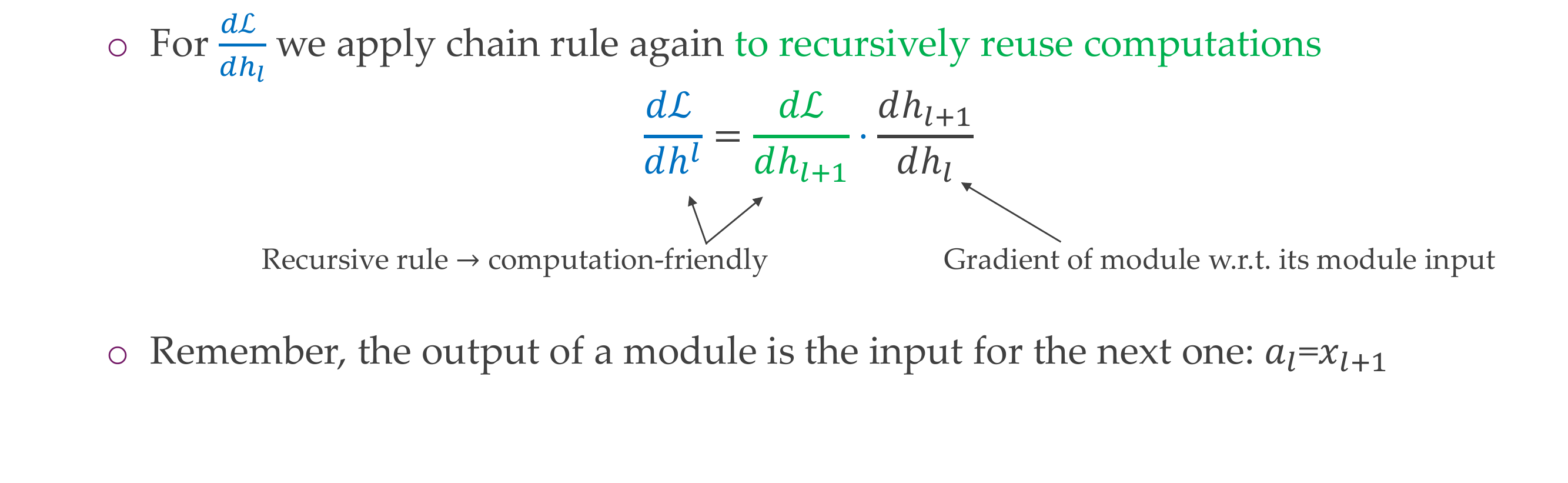
25.1 Backpropagation in summary
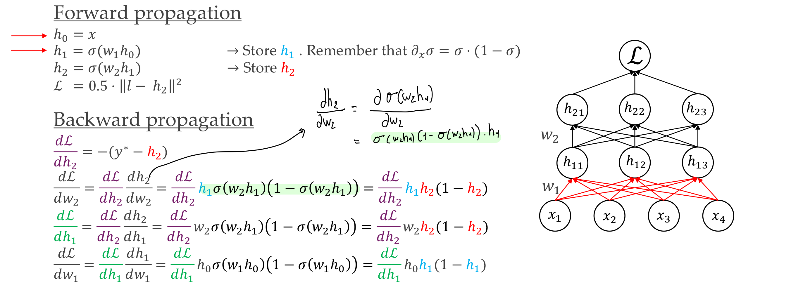
- Note: in the figure above, we know what is \(h_0\), \(h_1\), \(h_2\) and \(L\) because we have initialized our \(w_1\) and \(w_2\) and we also know how the sigmoid function works:
That means all these values are known so that when we calculate the derivatives below everything is know and then we can use SGD to update the weights
Then the derivatives wrt. \(w\) are:
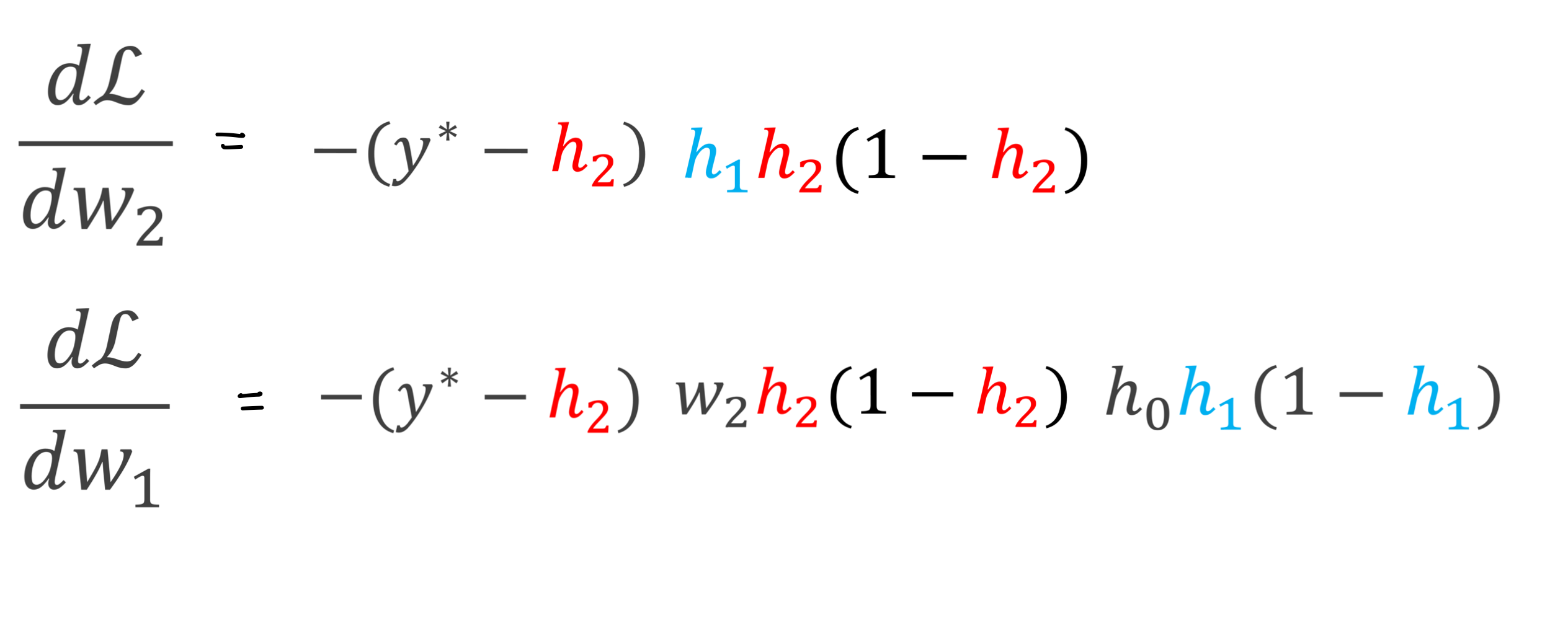
- These last equations is what we need to do SGD
Backprogation allows us to generally reduce the amount of space we need in order to compute all the gradients for all the layers, because storing the Jacobian takes a lot of space.
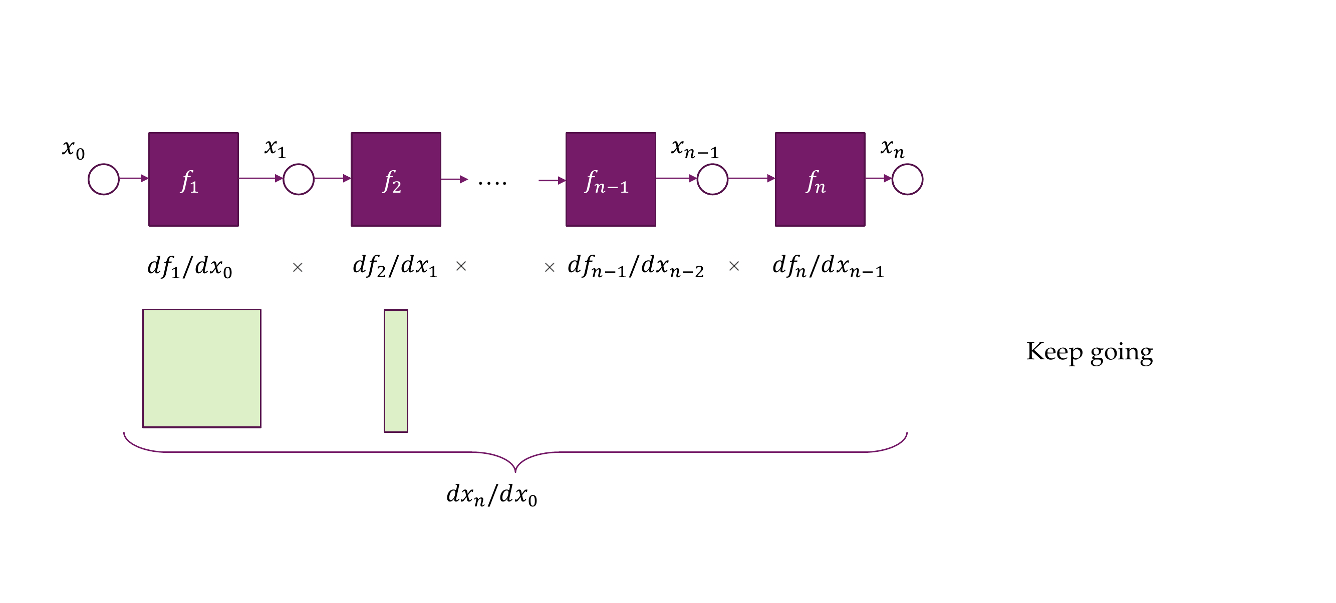
26 Chain rule visualized
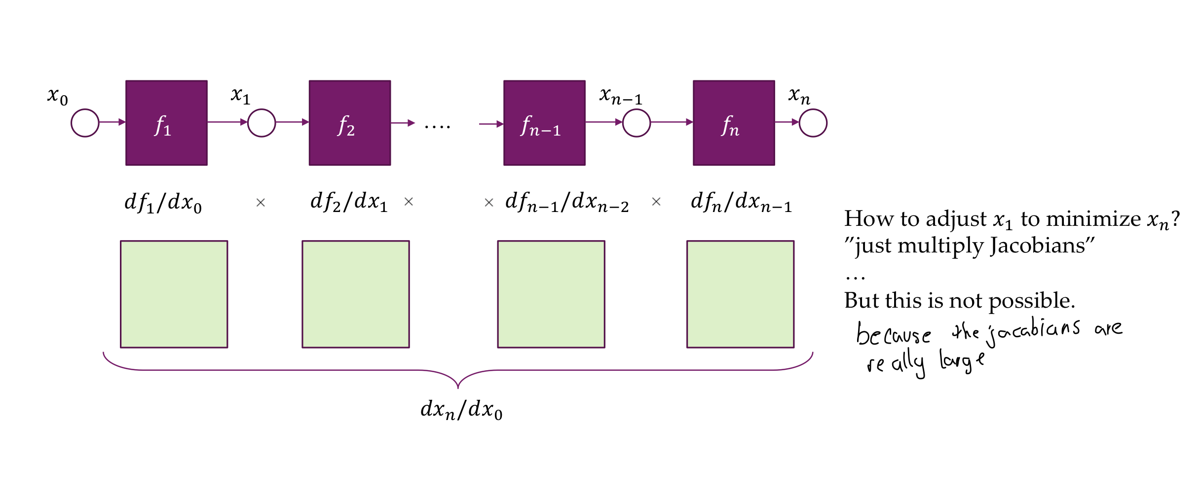
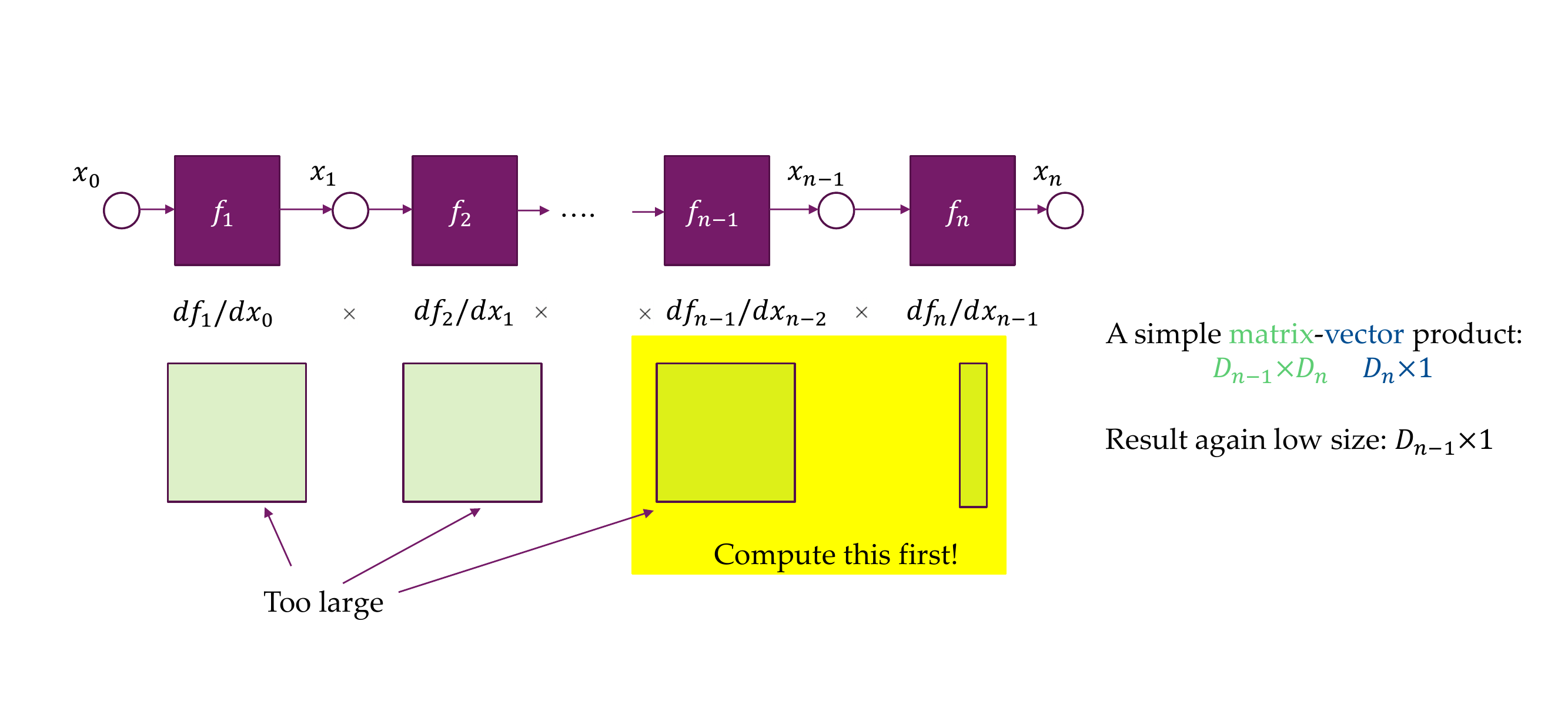
- But now if the ouput is an scalar, we get in the ouput a vector:
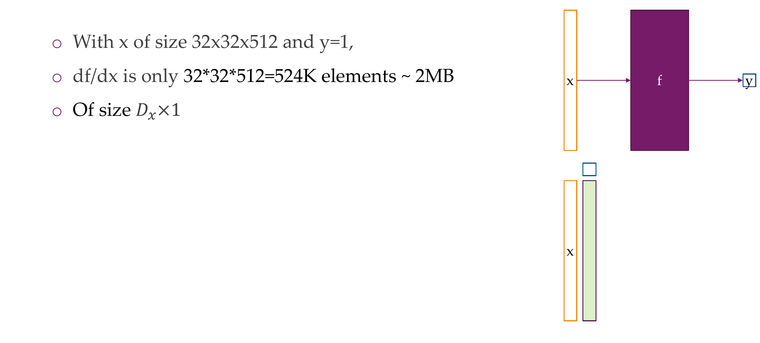
- Now from the back to front you are only multiplying vector times matrices instead of large matrices with large matrices
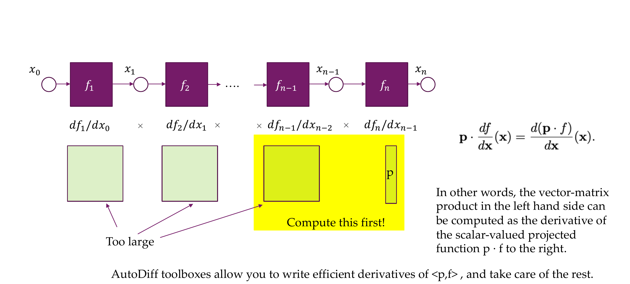
27 But we still need the Jacobian
28 Computational graphs: Forward graph
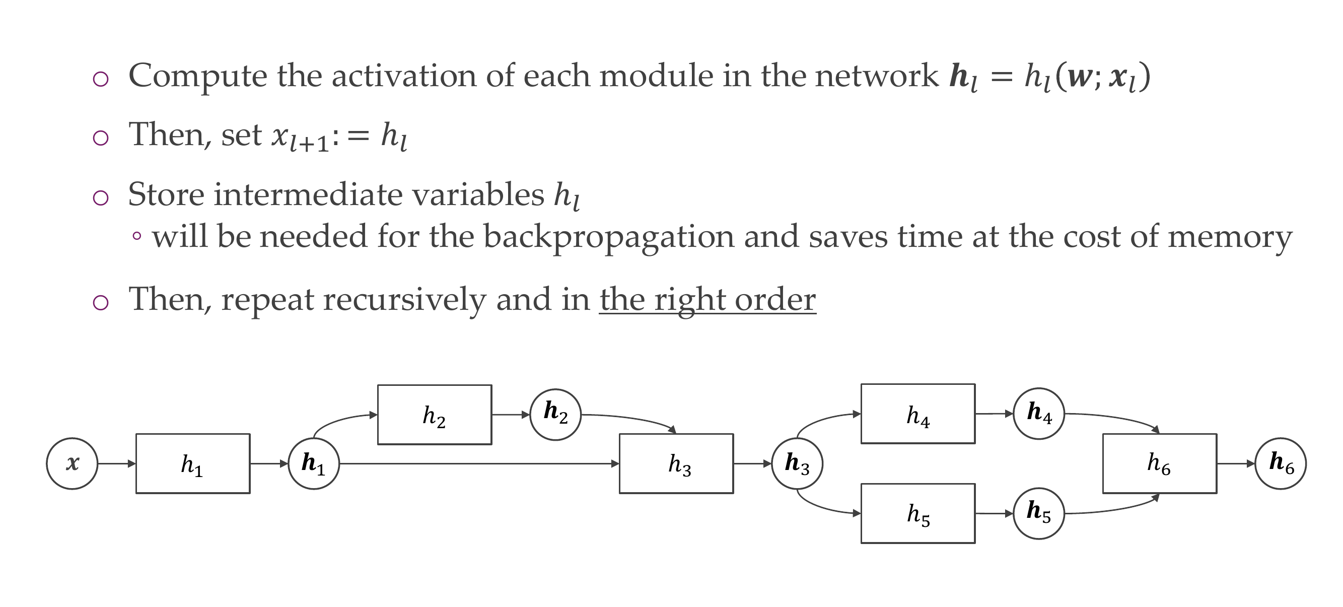
29 Computational graphs: Forward graph