1 Outline.
2 Semantics
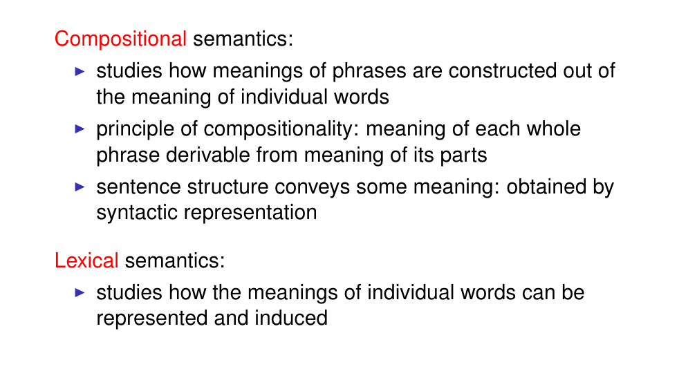
Semantics is concerned with modelling meaning
Compositional semantics: meaning of phrases
Lexical semantics: meaning of individuals words
3 What is lexical meaning?
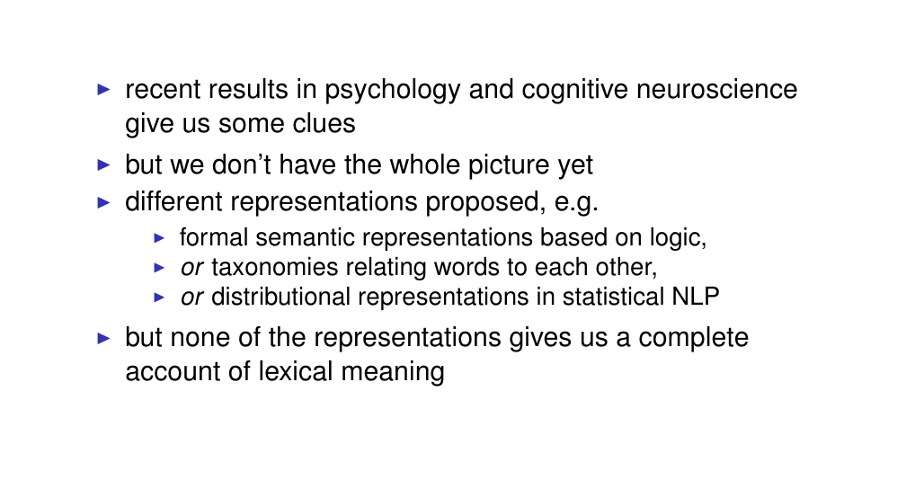
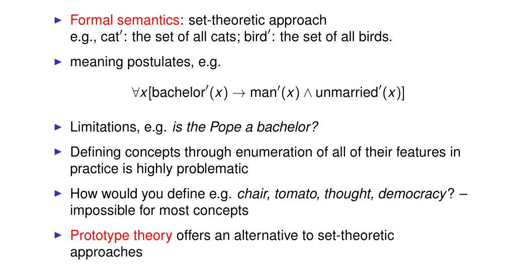
4 How to approach lexical meaning?
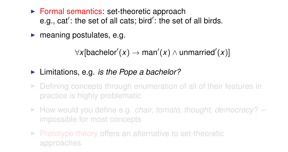
In formal semantics: The meaning of words are represented as sets
i.e Bachelors -> if is a man and also unmmaried
5 How to approach lexical meaning?
6 Prototype theory
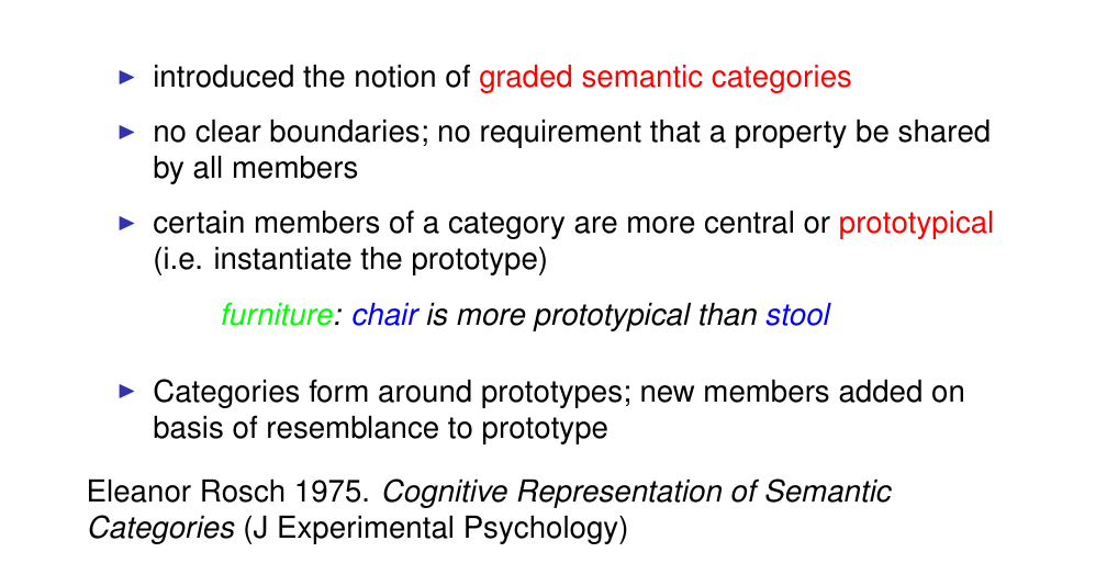
Prototype theory: concepts are represents as a graded category, it is like a human categorization
- not all members needs to share a property
i.e furniture -> chair is more central (prototypical) than stool or a couch
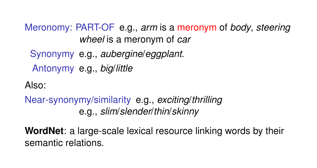
7 Semantic relations
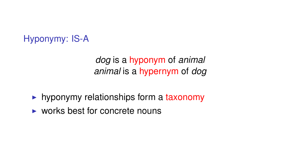
Taxonomy refers to the science of classification, specifically the classification of living organisms into various categories based on shared characteristics
8 Other semantic relations
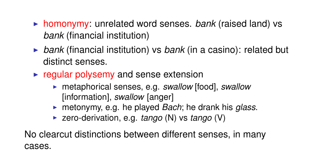
9 Polysemy and word senses
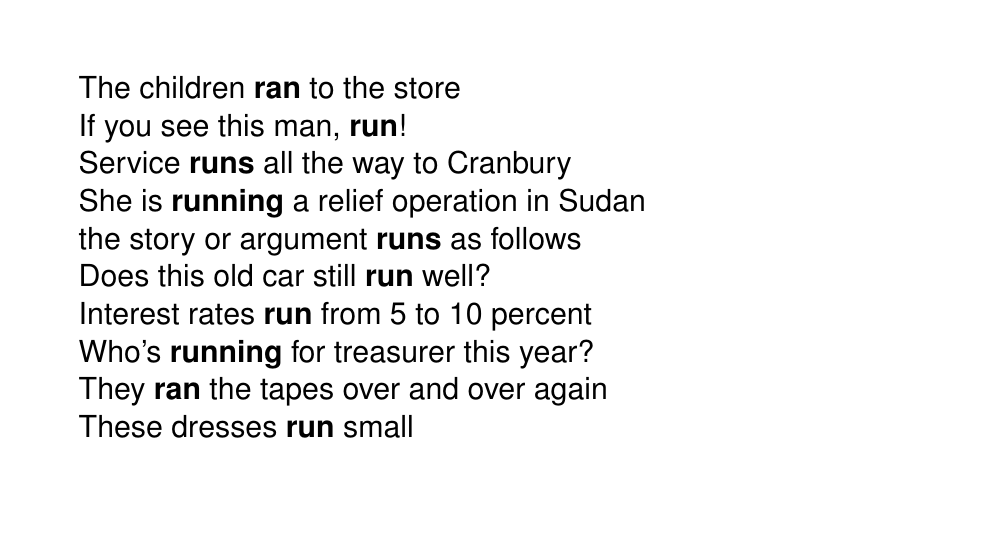
Polysemy is the ability of a word to have multiple meanings
A word can mean different things in a different context
10 Polysemy
11 Outline.
This a modeling framework
12 Distributional hypothesis
We can analysis the word depending of how it is used in a large corpus
A corpus (plural: corpora) refers to a large and structured set of texts,
13 Distributional hypothesis
14 Distributional hypothesis
15 Distributional hypothesis
16 Distributional hypothesis
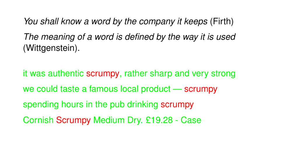
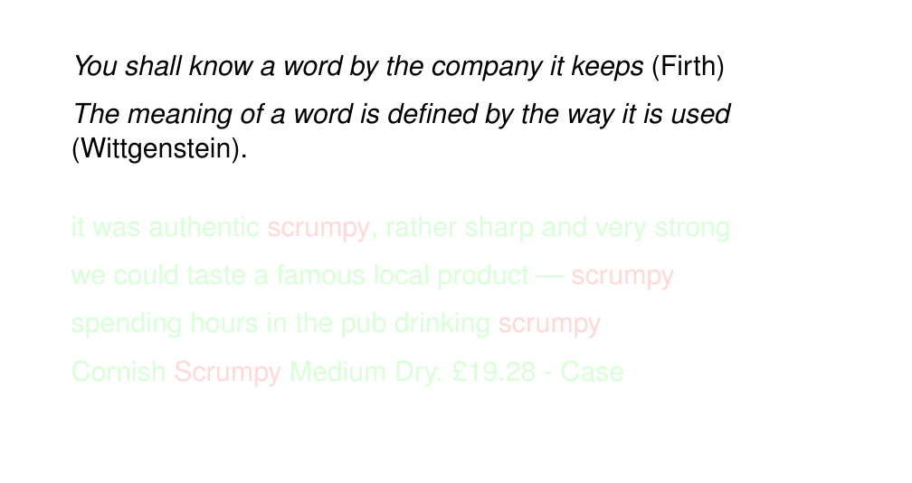
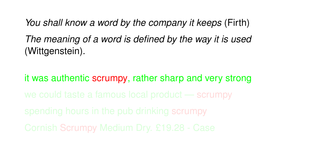
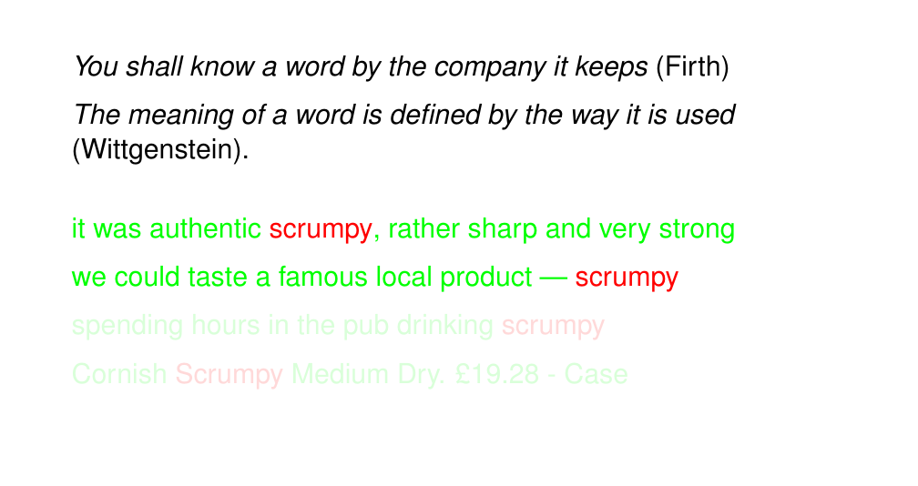
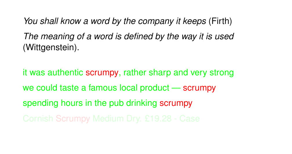
17 Scrumpy

18 Distributional hypothesis
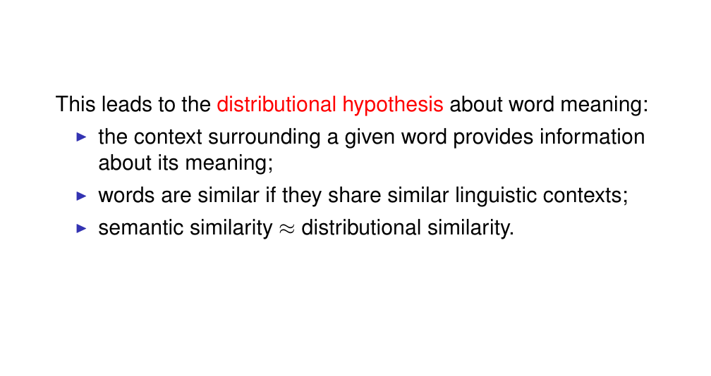
The context about a word provides the information about its meaning
Meaning similarity, could be then be the vector that is also similar to another where each element of the vector is a context, so the more similar context the closer the meaning
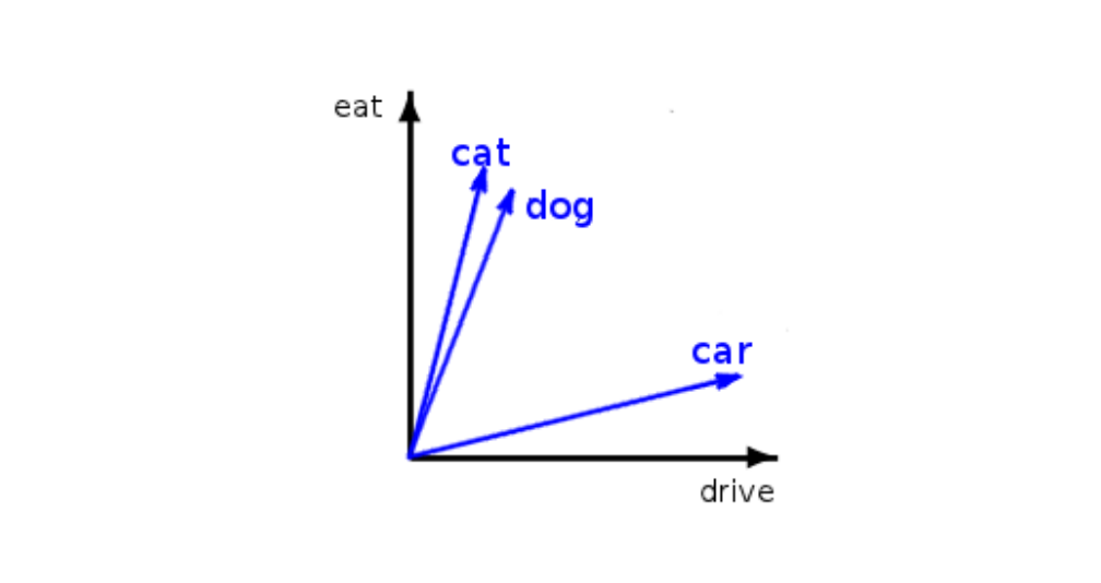
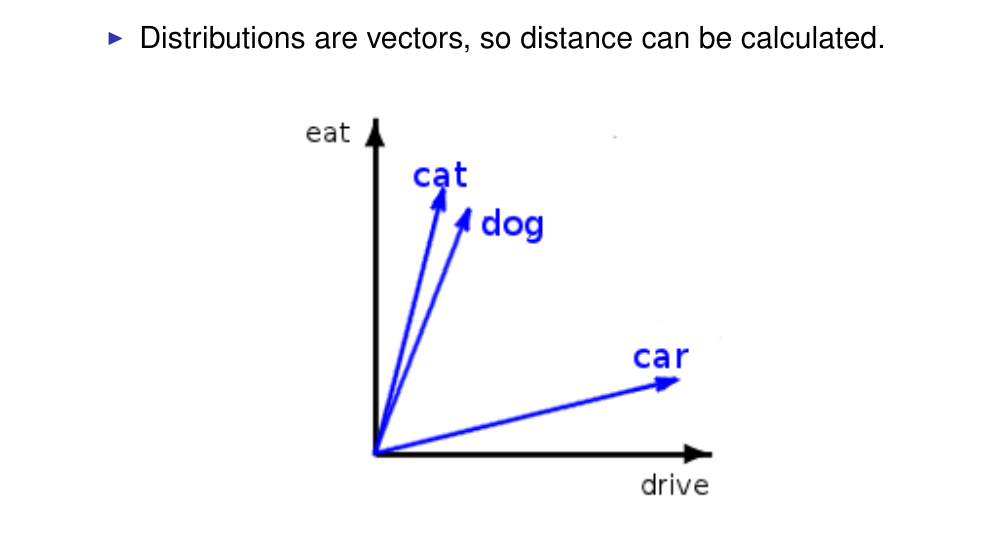
19 The general intuition
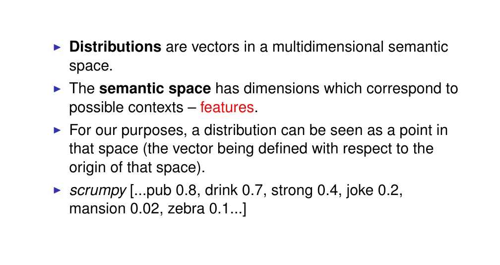
each word is a point: a row
Dimensions: are all possible contexts in our dataset
the values are the frequencies that ocurred in that context
20 Vectors
21 The notion of context
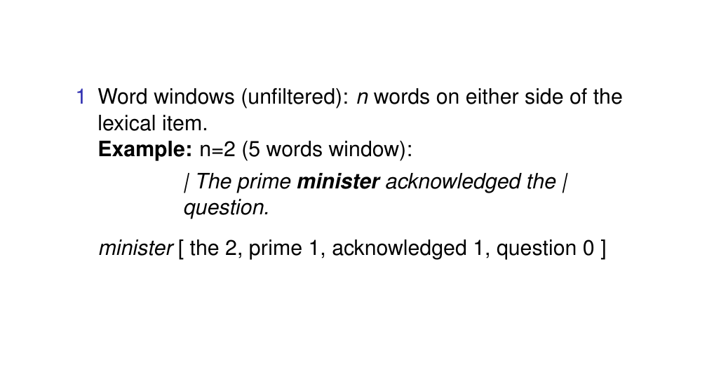
22 Context
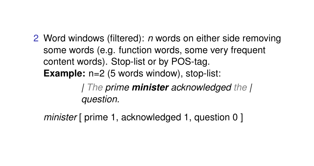
Here we delte words that are frequent
Here the window stays the same
23 Context
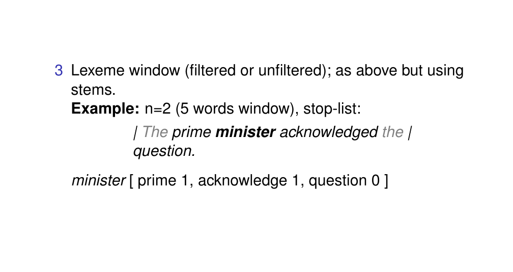
Now we just take the stem of each word and then we do a count on this stem words; here acknowledged -> acknowledge
This is handy if your corpus is not very large, because then your vectors would be very sparce meaning we would have zero entries because of the different variants of a word, so instead you want to aggregate context that mean the same so then we fix sparse vectors
24 Context
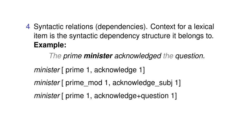
Instead of word window, we can use syntatic relations. That is we can extract syntactic context even for those words that are further way but have some relation with the wording that we are looking.
25 Context weighting
The first decision: how to model
The second: how to weight the context, so which metric we wil use
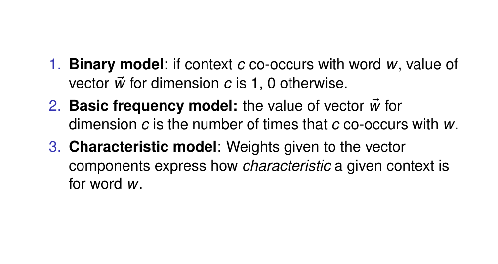
26 Characteristic model
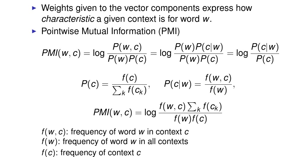
Here we are saying that there are some words that are more characteristic of a context. For i.e ‘floffy’ can be refered to dogs or cats, or toys but not so much of ‘computer’, ‘screwdriver’
It measures the joint probability of the word and the context (numerator) and the probability of them occurring together if they were independent (denominator)
P(c|w): how likely it is the context given that we are seeing this word.
So we want to compute the probability of the word occurance in the corpus to their probability of occurrence independently
27 What semantic space?
The first decision: how to model
The second: how to weight the context, so which metric we wil use
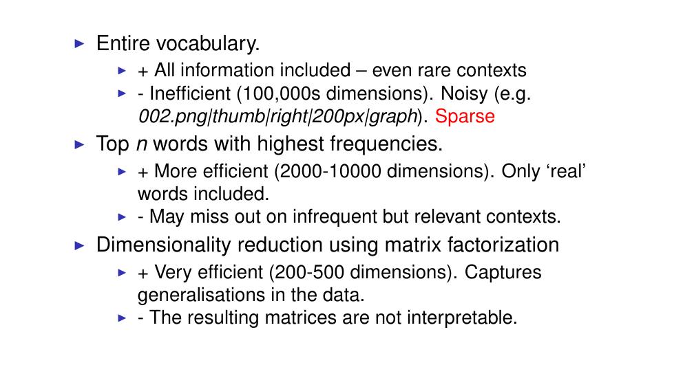
Third design decision: what kind of semantic space to use? aka how many context to include
- We can use entire vocabulary
A CON is that it will be very sparse if we use the whole vocab
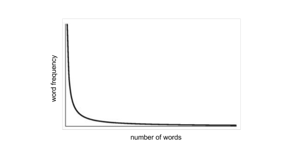
28 Word frequency: Zipfian distribution
29 What semantic space?
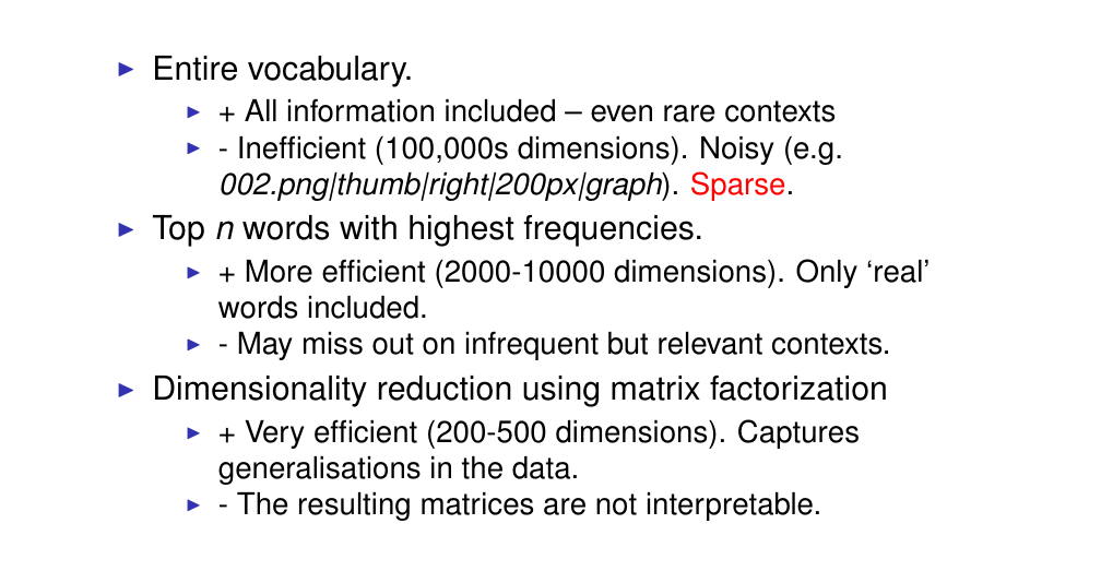
Dimensionality reduction is to benefit from approach 1 and 2
30 An example noun
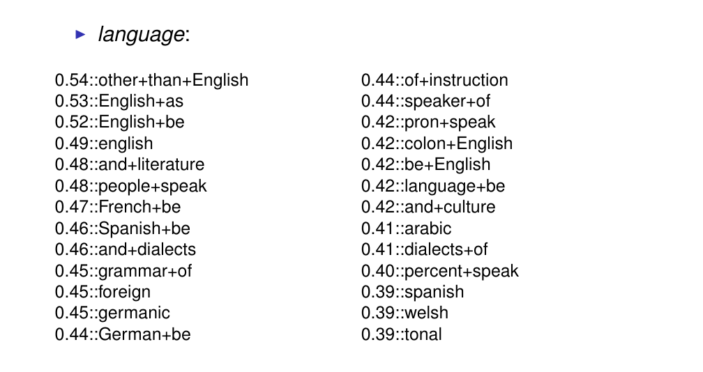
the values here are PMI values
31 An example adjective
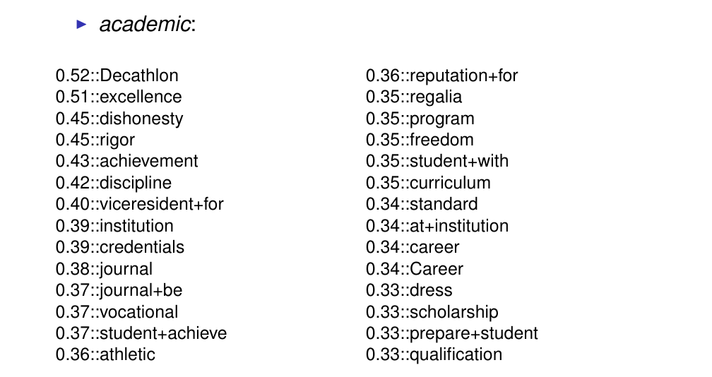
Decathlon is strange to see in the first place
PMI property: no matter which data you apply to is that you would get unreseanable PMI values for rare events.
So Decathlon is rare, and if it appears with academic once, then it will have a high PMI, because has a low prior probability
32 Polysemy
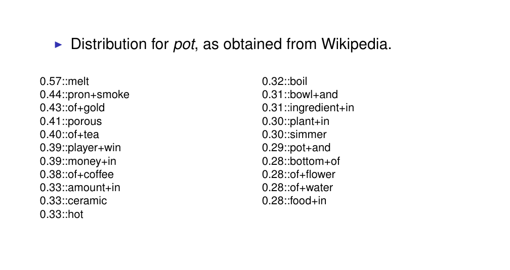
Polysemy is the ability of a word to have multiple meanings
All these senses are encoded and collapse toguether within a single distribution. Basically you have different context that correspond to different meanings and
33 Calculating similarity in a distributional space
34 Measuring similarity
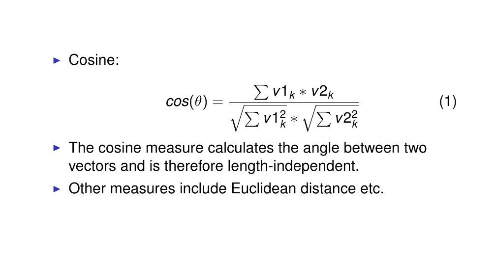
The dot product of the two vectors that is normalized by the vector lenght
The Euclidean distance considers the length of the vectors:
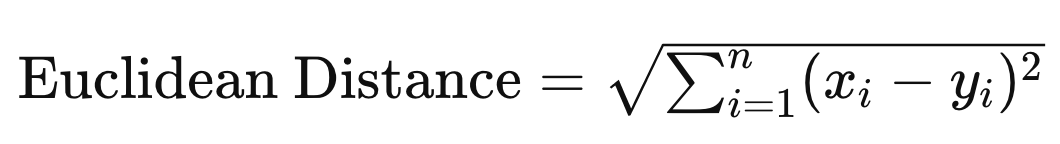
The euclidean distance would be quite large, so that is why we need to normalize
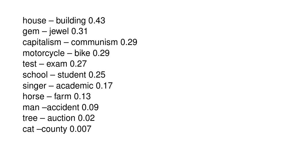
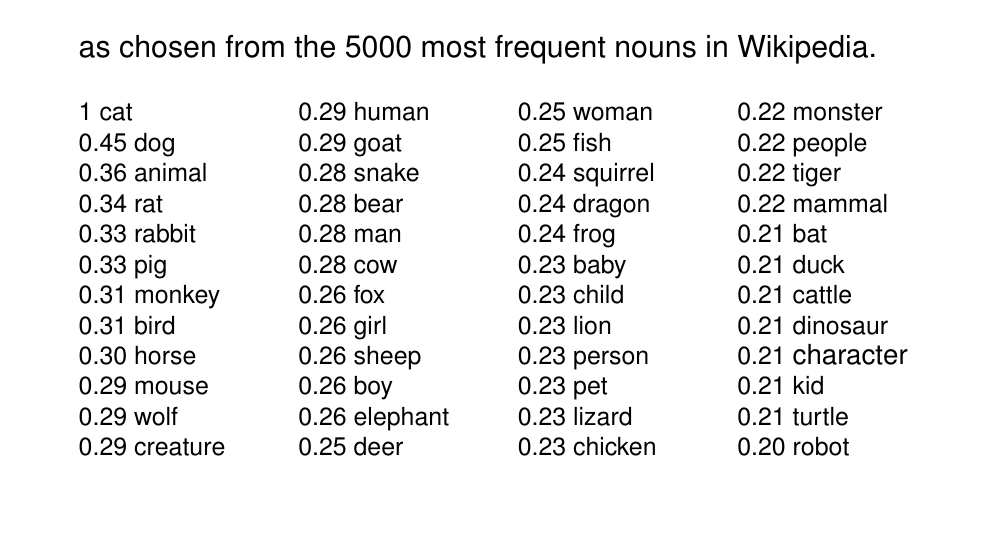
35 The scale of similarity: some examples
36 Words most similar to cat
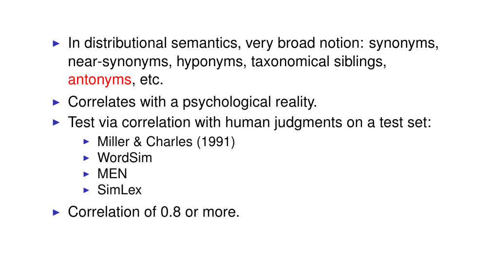
37 But what is similarity?
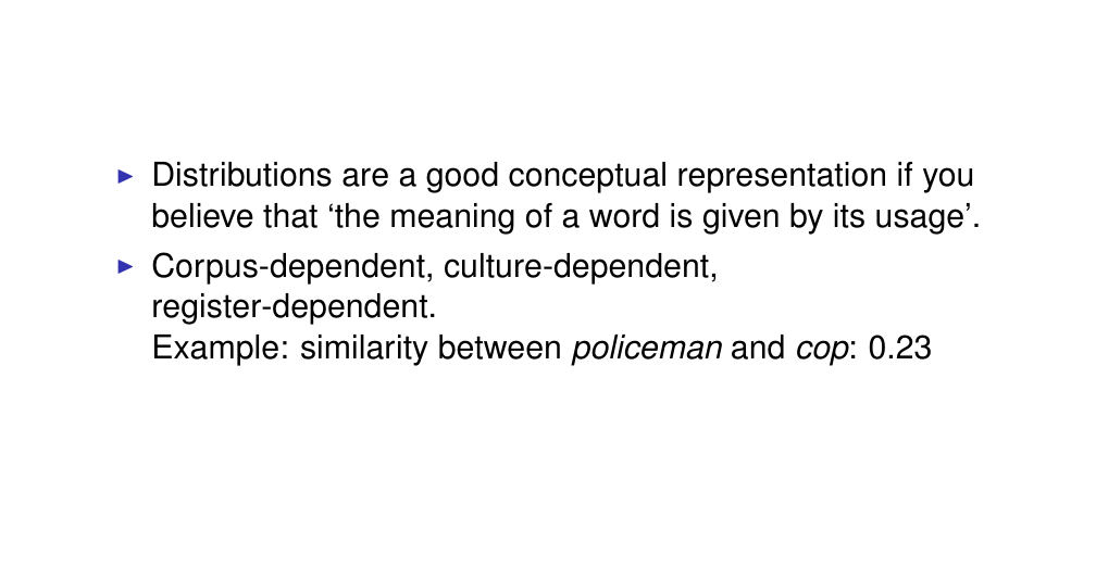
38 Distributional methods are a usage representation
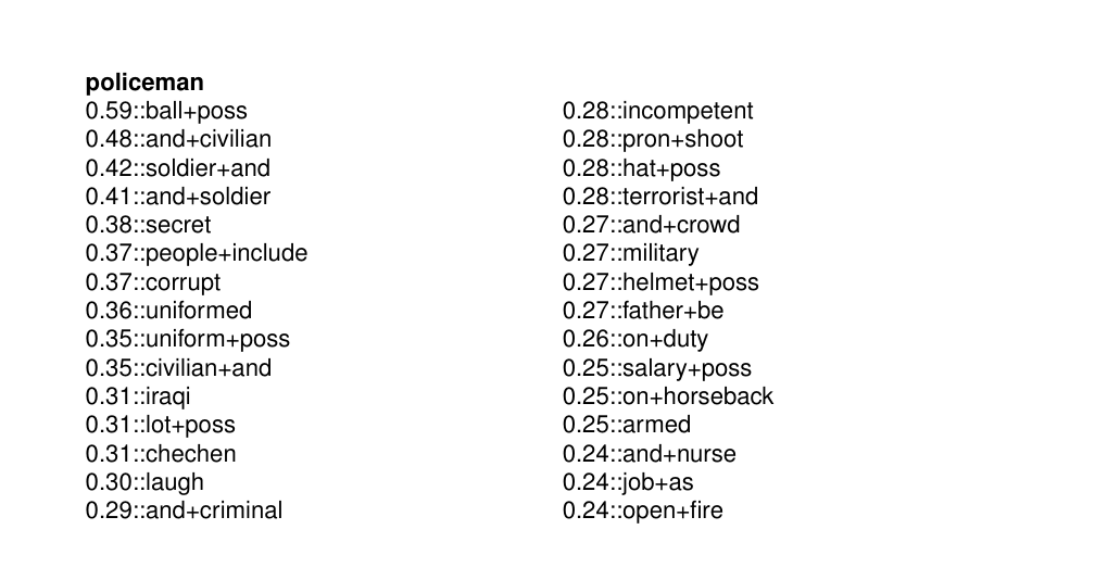
39 Distribution for policeman
40 Distribution for cop
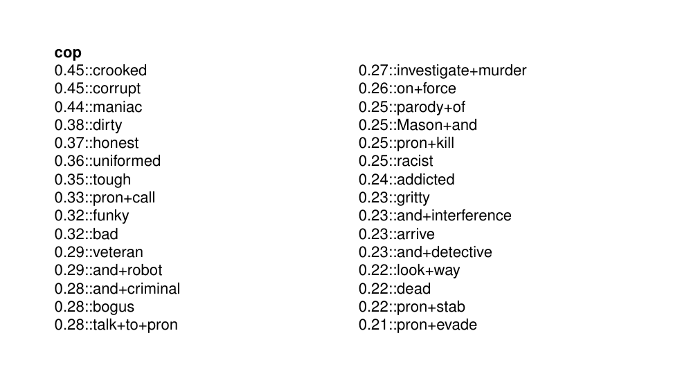
Cop and policeman, even though the words seems to be the same, there is cultural associations with cop that is highly negative.
This means that words have relative meanings to the culture and thus if compared this terms between cultures their meanings could be totally different which then evaluating a similarity metric will yield that they are not similar.
Tha being, we take two words from the same corpus but because of cultural use of words they may have different distributions (cognotations). Unquestionable, this is a property of the data.
1set carriage bike vehicle train truck lorry coach taxi – official officer inspector journalist detective constable policeman reporter – sister daughter parent relative lover cousin friend wife mother husband brother father
2set car engine petrol road driver wheel trip steering seat fo, highway sign speed - concert singer stage light music show audience performance ticket - experiment research scientist paper result publication laboratory finding
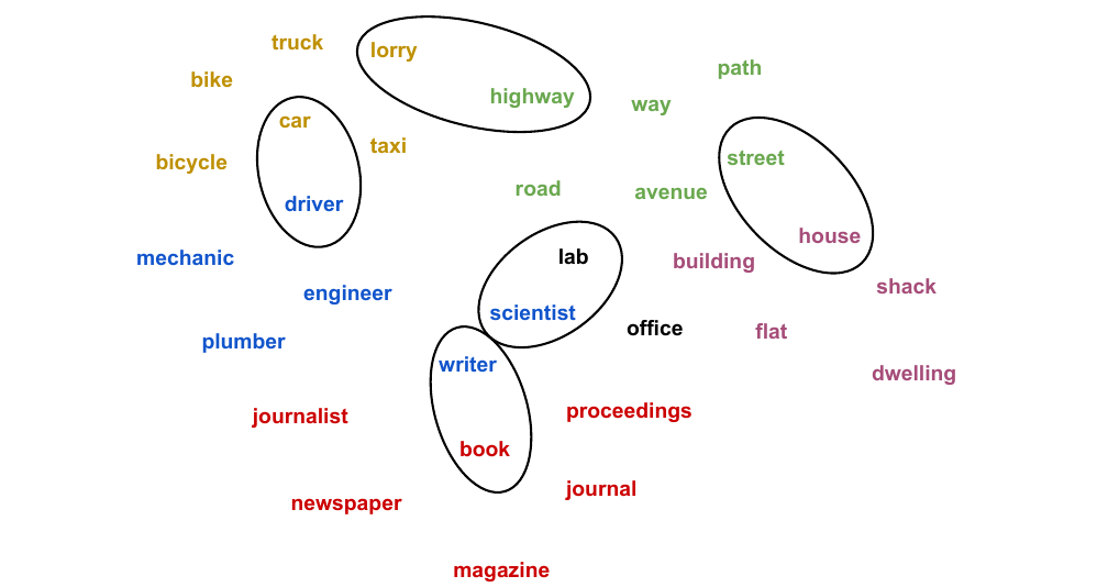
41 Clustering nouns
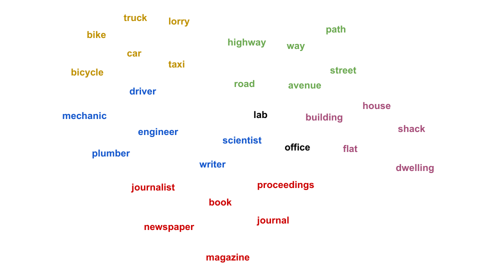
42 Clustering nouns
43 Outline.
44 Distributional semantic models
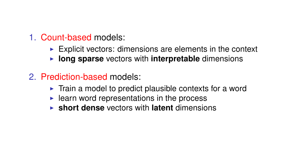
Dense vectors or word embeddings
Count-based models we can see clearly
Here we train the model to predict what makes a good context for a word.
Dense in the sense that the dimensionals are used and there are fewer dimensions, the model learns some interactions between them. However the dimensions are latent so if the model has a strange behaviour is very hard to know why.
45 Sparse vs. dense vectors
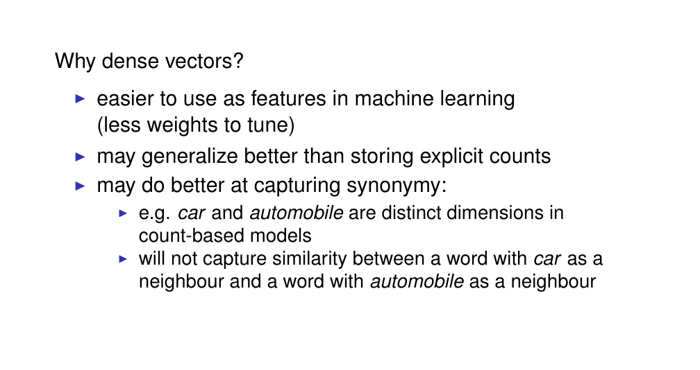
In traditional distribution models we can have tends of thousands of contexts in a large corpus
they generalize better, by having those latent dimensions that are trained in the prediction task, the model learns to map similar context toguether to the same dimensions.
If in a traditional distribution model you would have distints concepts for car and automobile, there is no way for the model to know that they provide the same information, whereas in a dense vector we can agregate over similar context, you can map them to the same dimension and you can reduce the redundancy in the data but also end up with a model that is more generalizable
46 Prediction-based distributional models
The most popular model of word embedding of prediction base is the Skip-gram model
Probabilistic language models, such as n-gram models where our goal is given a sequence of words we want to predict the next word that comes next
Here, the task is the same exceot that we use a NN to perform this prediction.
The idea is that we can learn word representations in the process
47 Skip-gram
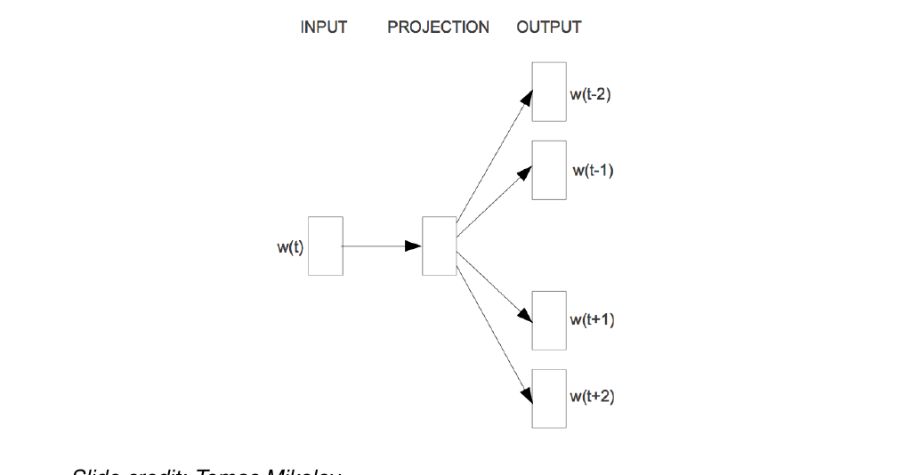
in Skip-gram we do not care about the sequence, but rather we want to take individual words as input, and we want to output the words that it can occur in the data i.e. if we take a 5-word window, basically we want to train the model to predict the valid context for thee word and then we lear the world representation in the process (in the projection layer)
48 Skip-gram
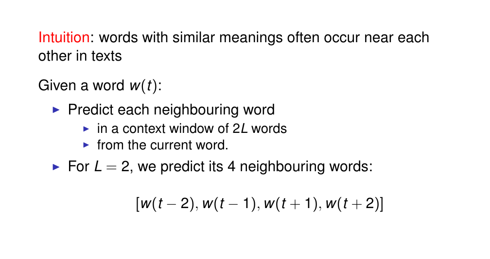
Words that occur toguether in the data should have some similarity in meaning. This is different from i.e we compare context towards the current and the relation in their similar meaning but rather a word should be similar in meaning to its neighbors.
Essentially we want to compare the vectors of the word and their neighbors
Given word at time t
Goal: predict all its neighboring words within a window. For instance we use a 5-word windows then these are the words to predict
49 Skip-gram: Parameter matrices
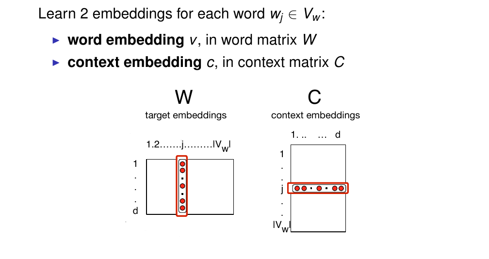
For each word skip gram learns 2 parameter vectors:
For each word it learns two vectors:
The word vector, that is the word embedding v, in word matrix W
This is the vector that represents the meaning of that wordA context vector that is the vector that represents its behavior as context for other words
In a sense each word can have two rows: it can act as a word from which we are learning the word meaning AND it can also act as context for other words
W: is the matrix of word embeddings
C: the matrix of context embeddings
and so then we choose the dimensionality of our embeddings to have, for instance between 50 and 500 dimensions
Here for a whole Vocabulary we have a vector for every word, so the dimensionality here is the size of our vocabulary, so the columns are the word embeddings for all of our words
Again:
W:
So in the columns we have the vector oer word so we go from 1..Vw
The rows represent the dimensionality of the vector
C:
The columns are the dimensions
The rows we have the size of our vocabulary so we have a word, so the number of rows are the number of word in the vocabulary
In practice, these are the same, so we say we use individual words as context, so all words will learn embeddings, and each word can acts as a context. However there is no requirement to be the same, in fact the context vocabulary can be different and we can use any definition of context as we discuss in distributional models
50 Skip-gram: Setup
we go word by word extracting its context.
This may look like Bigram prob but is not, and is not because position does not matter. So basically we consider each context in isolation like a set, so the context that the word might have and we operate over context pairs, the order does not matter in the sequence. So word and each context in isolation. And which context are possible we define based on the word window for any other criteria like we explain before like:
- Context window unfilter
- Context window filtered
- Context window lexeme filtered
- Connected by a grammatical relation
So the position of the context does not matter once we have extracted the context but of course it does matter in the process of extracting it, so it has to be whithin the word window
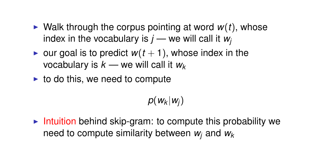
Intuition of skip-gram: to compute that probability we need to compute the similarity between w_j and w_k
51 Skip-gram: Computing similarity
52 Skip-gram: Similarity as dot product
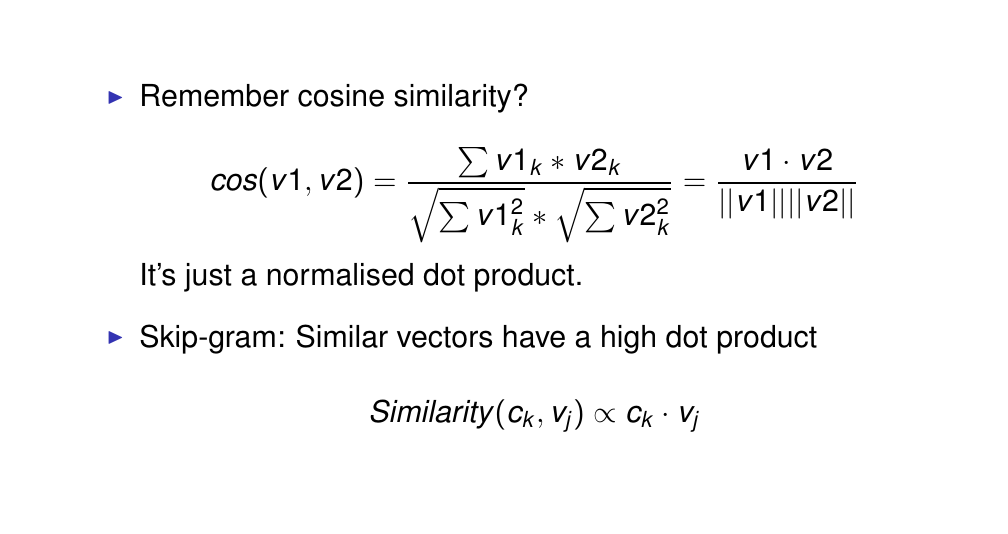
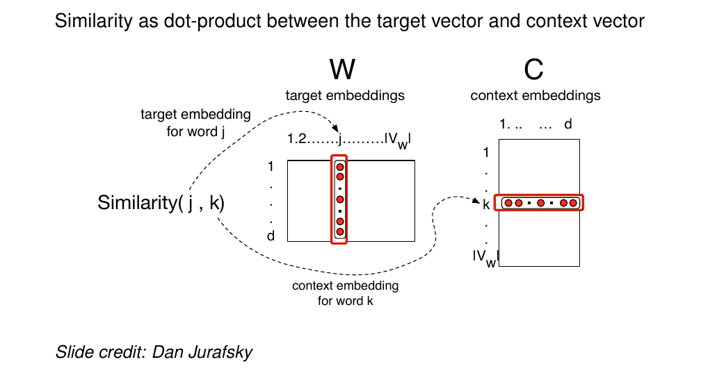
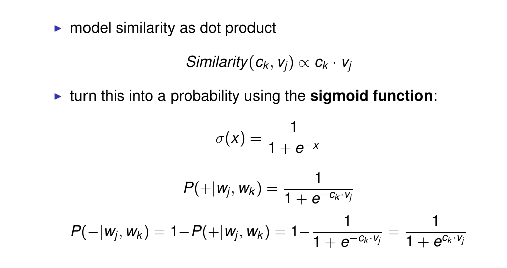
Why do we use dot product to compute the similarity. Again we use cosine, here we used it because it does not matter about the mangnitude but if they are pointing in the same direction then they are considered similar.
So vectors that are similar in this case w_j (current word) and w_k (word to predict) will be similar if they have a high dot product
53 Skip-gram: Compute probabilities
case w_j (current word) and w_k (word to predict) v_j (current word) and c_k (word to predict)
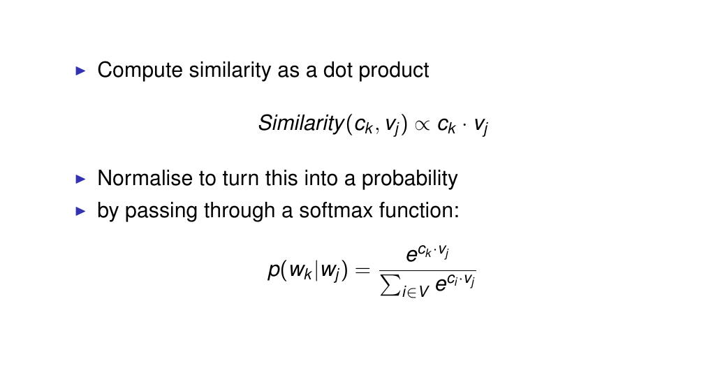
So here P(w_k|w_j) we want to predict how likely is that this context is predicted.
We end up with having a vector of dot products, so we are comparing the word with all of the context vectors, that gives a vector of products over the whole vocabulary and then we normalize it using softmax
At the end we use softmax to make probabilities summ up to one
54 Skip-gram: Learning
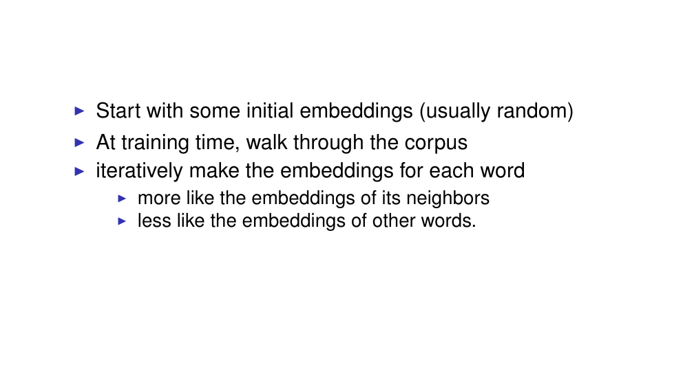
we iterative update the embeddings to make the embeddings of our words more similar to the real seen context words and less similar to the embeddings of everything else (other context words)
55 Skip-gram: Objective
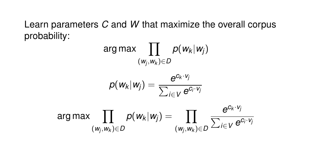
So we want to maximize the overall corpus probability, that is the probability of the real seen context.
Here we assume that the context is independent of each other, so the whole sequence does not matter. We assume that the probabilities are independent of each other and so basically the objective becomes to maximize the product of the probabilities of the real seen context pairs
Where:
- c_k is the vector representation of the context word w_k
- v_j is the vector representation of the word w_j
56 Visualising skip-gram as a network

our input here is the vector representation of the word
The last layer tell us all the possible contexts.
So we are predicting a context word at a time. For ie. here w_t is a vector and we predict all the probabilities of context words
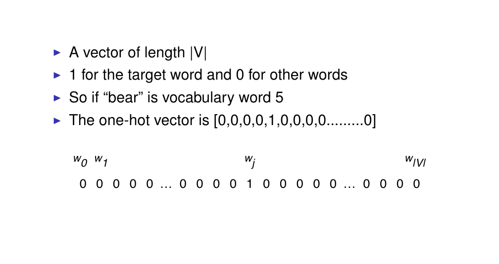
57 One hot vectors
58 Visualising skip-gram as a network
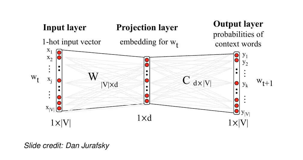
The problem arises at computing softmax. If our corpus is large then the denominator will go over this large text thus being computationally expensive. So basically we have to iterate over all the vocabulary to perform the update
59 Skip-gram with negative sampling
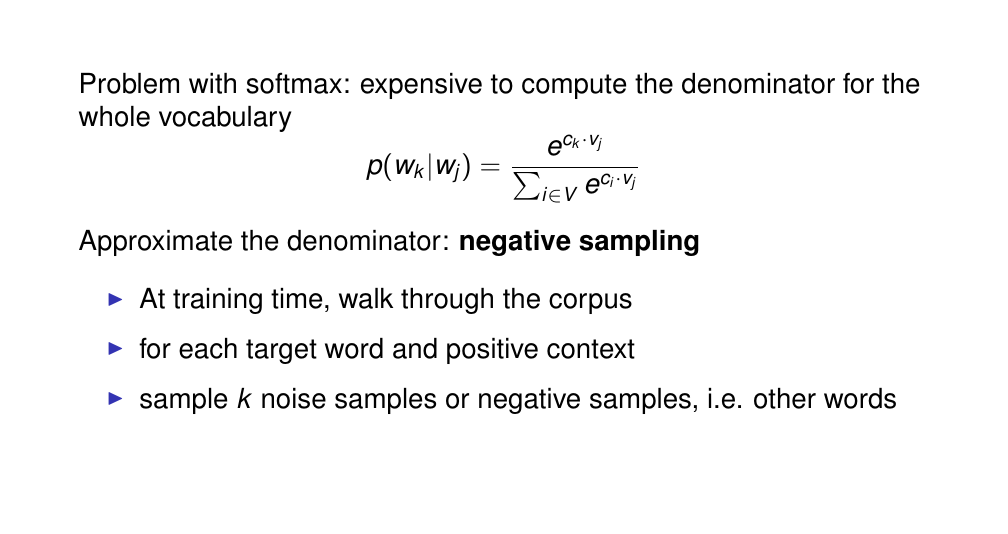
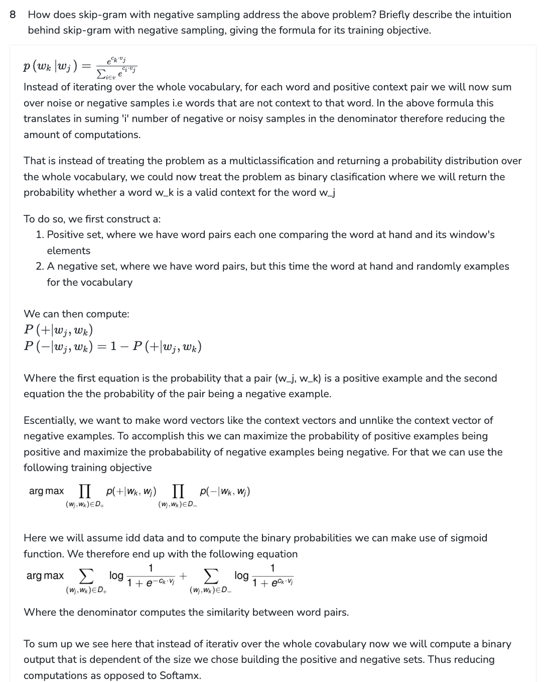
Instead of iterating over the whole vocabulary, for each word and positive context pair we will now sum over noise or negative samples i.e words that are not context to that word. In the above formula this translates in suming ‘i’ number of negative or noisy samples in the denominator therefore reducing the amount of computations.
60 Skip-gram with negative sampling
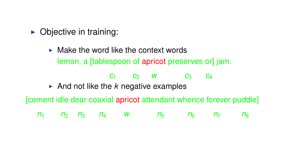
For each word of the window: so for word pair (‘tablespppon’, ‘apricot’), we are gonna randomly sample some negative examples, so sampling other possible contexts. You can decide how many you want to have per possitve context i.e 2 or 10. Say we are going to choose randomly two noise examples i.e ‘cement’ and ‘iddle’, those are words that have nothing to do with ‘apricot’ so those are the negative examples.
How to choose negative examples? it is just random and it is done over the whole vocabulary but you could be more especific and i.e pick from their unigram probability with more frequent words
So here if we take 2 negative examples per positive we will have 8 different pairs because our windows is 4
61 Skip-gram with negative sampling: Training examples
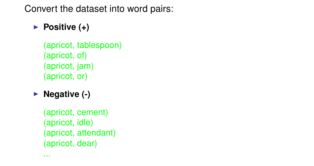
So basically we will convert our dataset into word pairs
62 Skip-gram with negative sampling
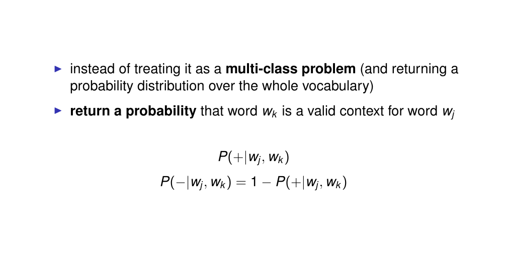
So now for a given pair we are going to predict if it is a negative or positive example, basically we converted into a binary clarification problem
So basically we will have a probability that a pair (w_j: context, w_k: example) is a positive example and then the probability that is a negative example.
63 Skip-gram with negative sampling
64 Skip-gram with negative sampling: Objective
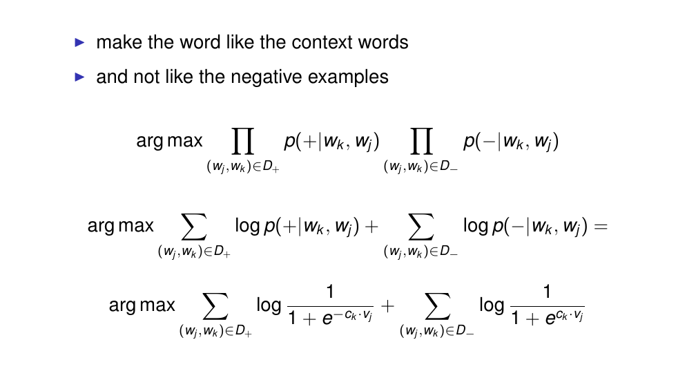
So now the intuition is that we want to make the word vector like the context vector and unlike the context vector of the negative examples.
So here we want to maximize the probability of positive examples being positive and maximize the probability of negative examples being negative
64.1 Savings from negative Skip-gram. Softmax –> Sigmoid
Edit:
To sum up we see from the last equation that instead of iterating over the whole vocabulary, now we will maximize over the positive and negative sets which their size is a design choice that as explained during the lectures is more computational efficient (less dot products to compute) as iterating over the whole vocabulary as it was the case with Softamx.
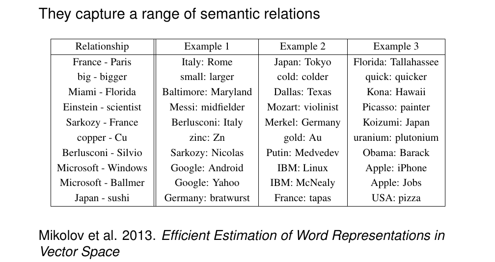
65 Properties of embeddings
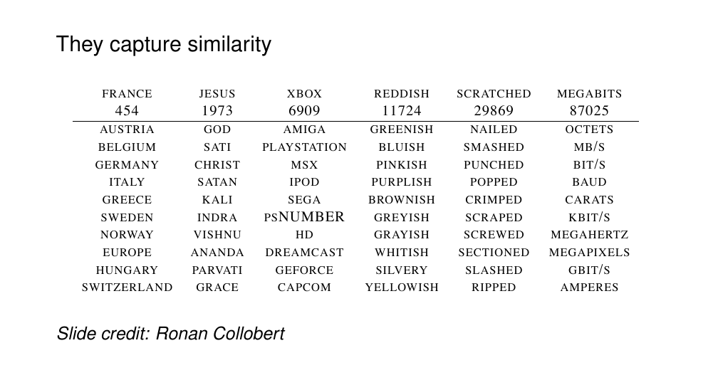
The number below France is the ranking of most similar words. The interesting thing is that if you do not use lexematitation, it also captures more find grained aspects of meaning. For instance in ‘Reddish’ we do not get other colors but we also get a red-like similar words is not about ish words because we also get silvery. This show us that the model cna capture fine grained aspects, which is what we want.
66 Properties of embeddings
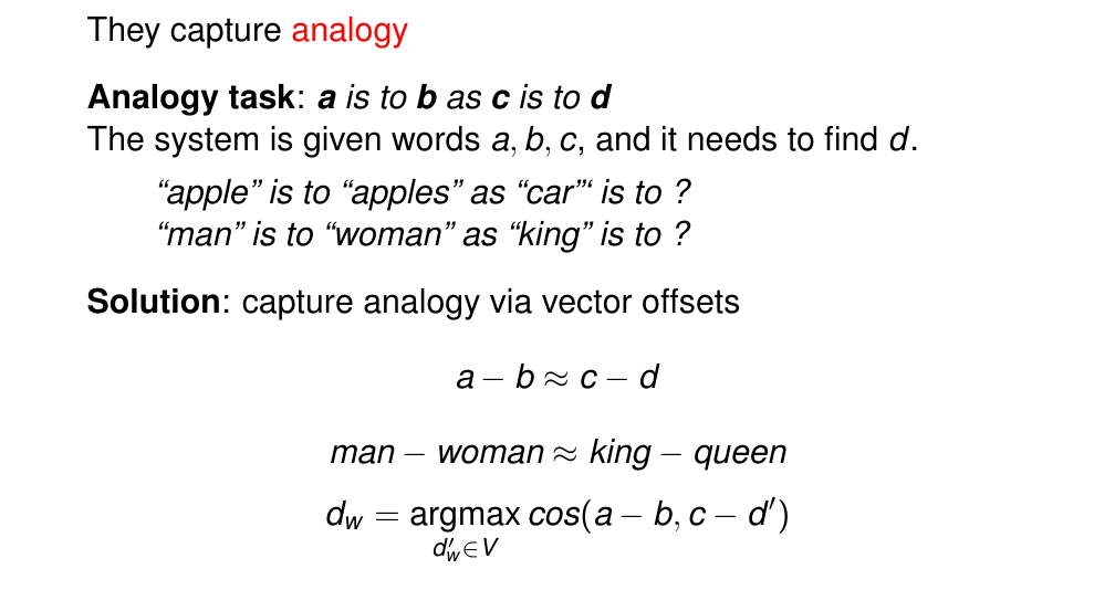
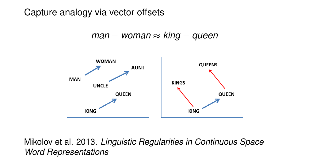
We compare two pairs of words in terms of their relation
- here in apples in the plural relation
- here in man and woman there is a gender relation
So the model needs to complete the analogy given a is b and then given c is to what?
67 Properties of embeddings
68 Properties of embeddings
69 Word embeddings in practice
In your NN the first layer are going to be the word embeddings which are some representations of the word in a sequence
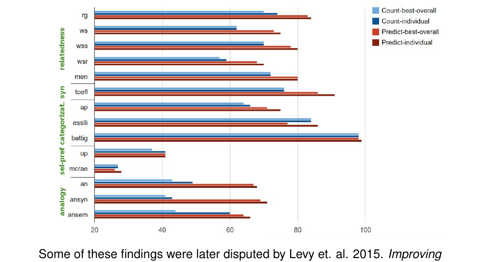
70 Count-based models vs. skip-gram word embeddings
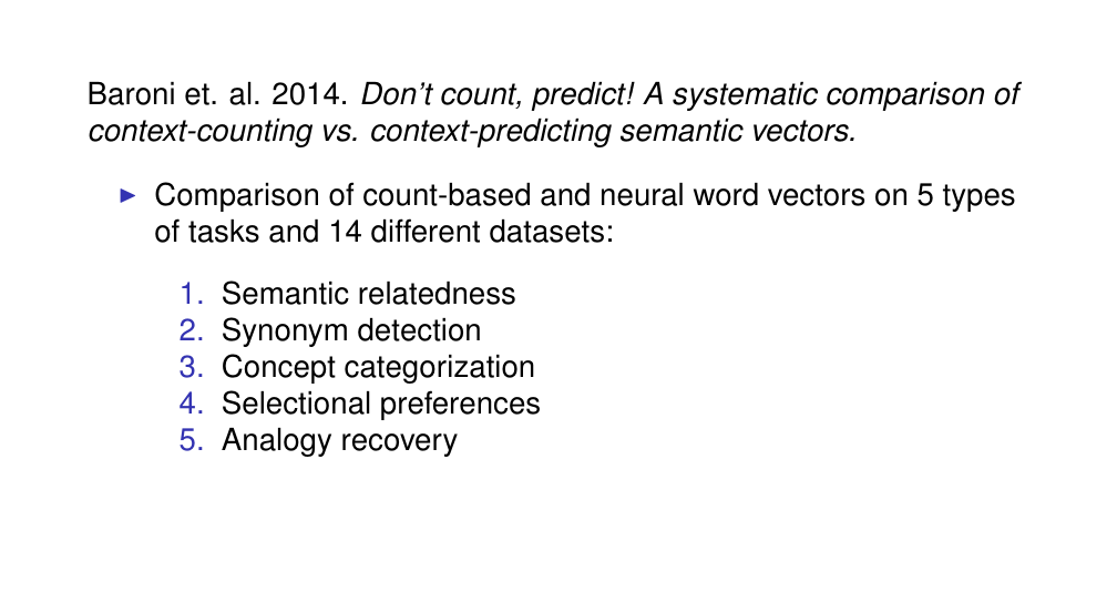
71 Count-based models vs. skip-gram word embeddings
72 Acknowledgement