Equivariances & Graphical Neural Networks

Description of this Post

1 Title

Slide 1

2 Organisation

Slide 2

3 Lecture overview

Slide 3

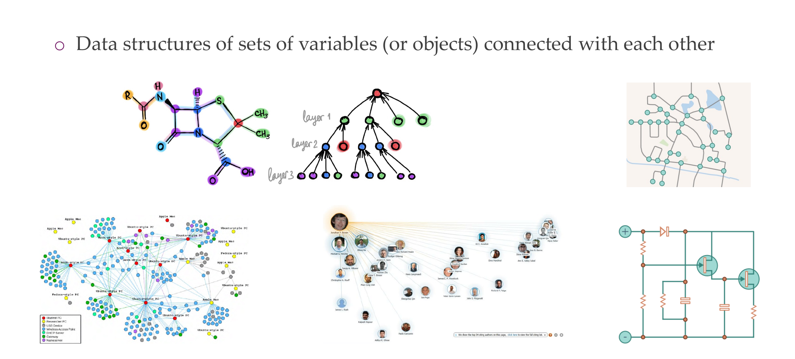
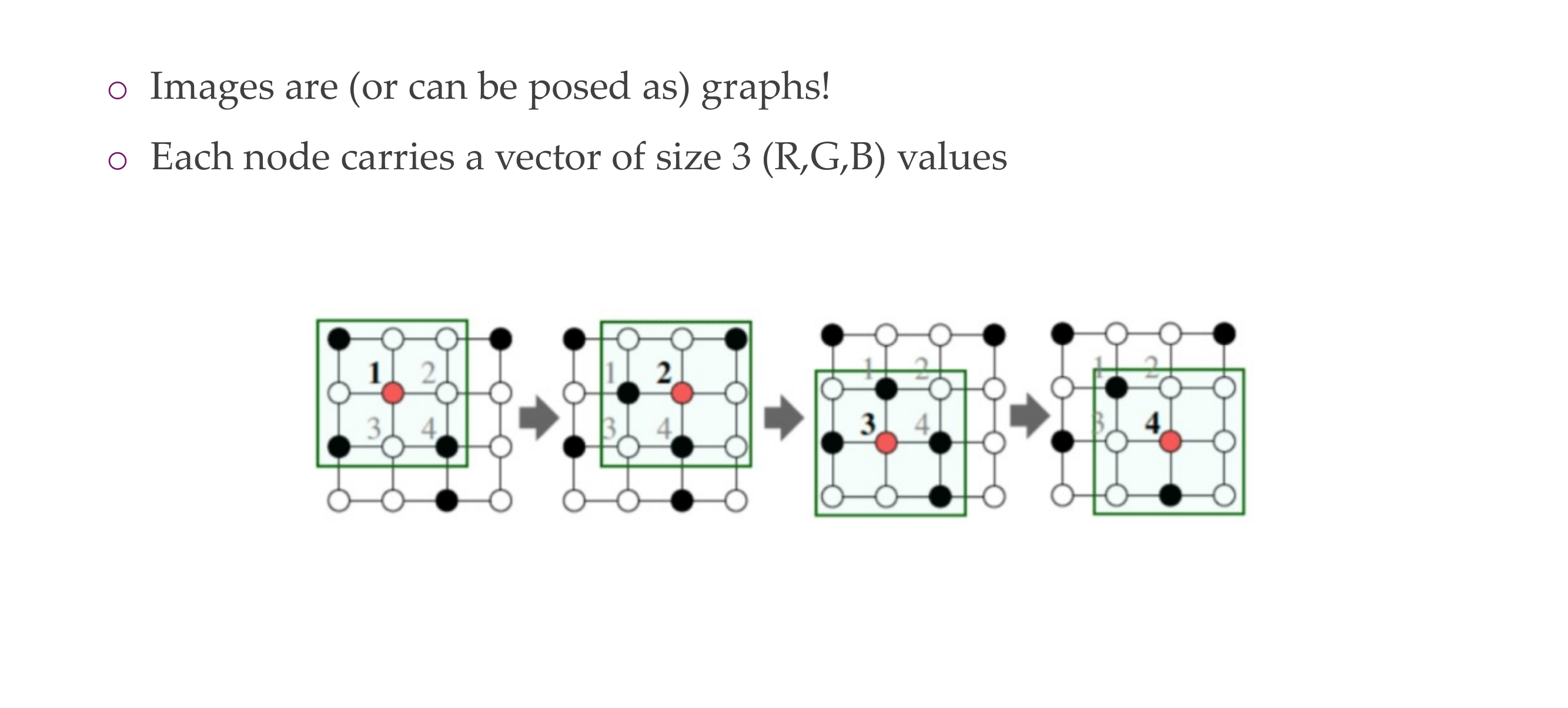
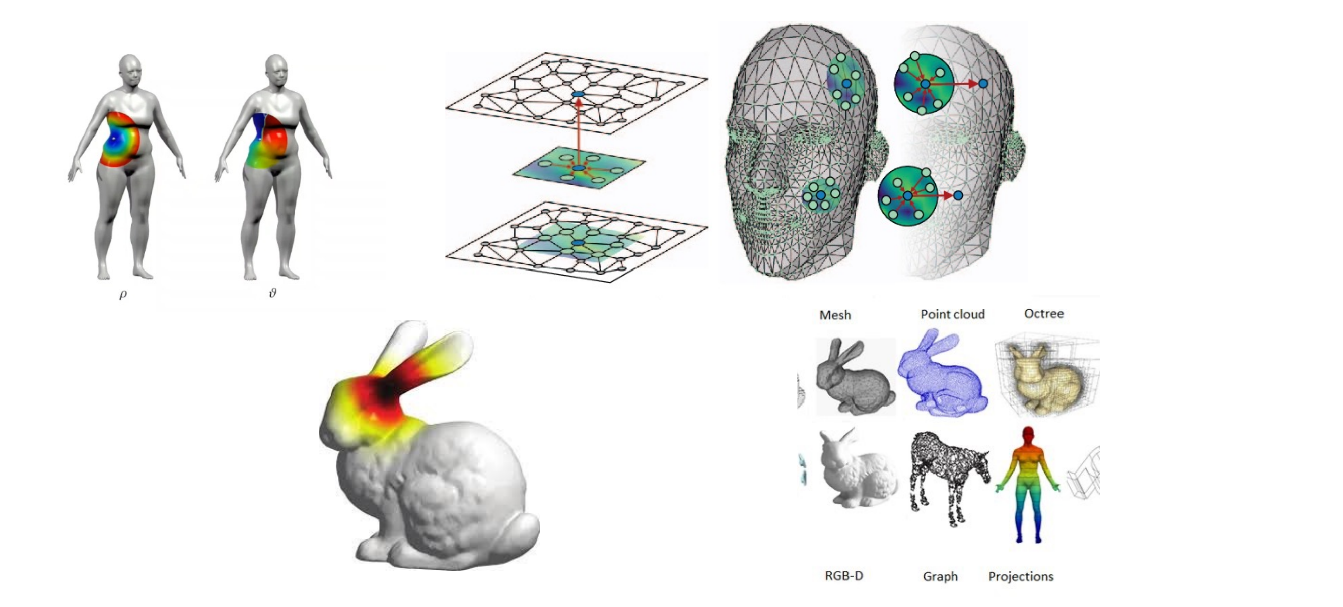
4 Graphs! They’re everywhere

Slide 4

5 What are graphs?

Slide 5

6 What are graphs?

Slide 6

7 Graphs as geometry.

Slide 7

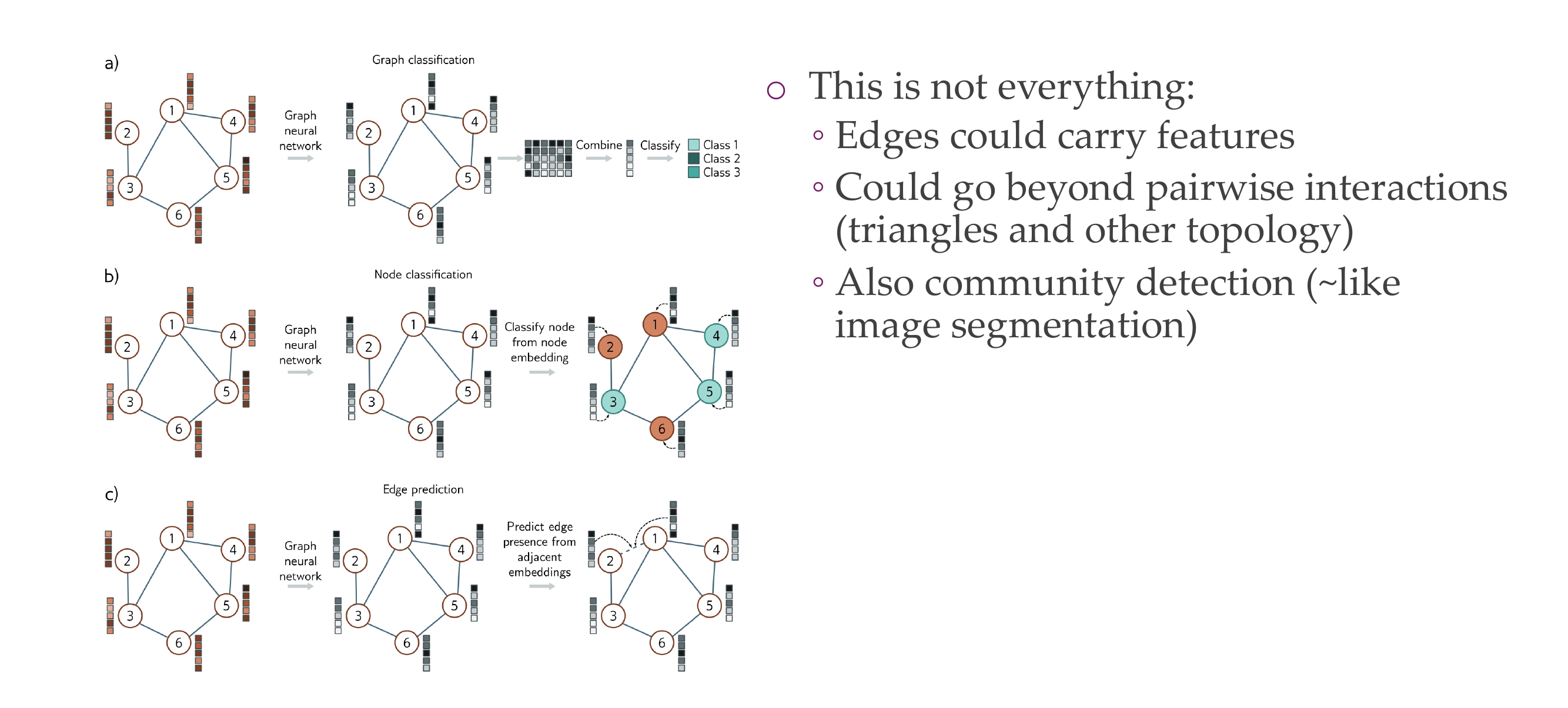
8 1) Classifying graphs

Slide 8

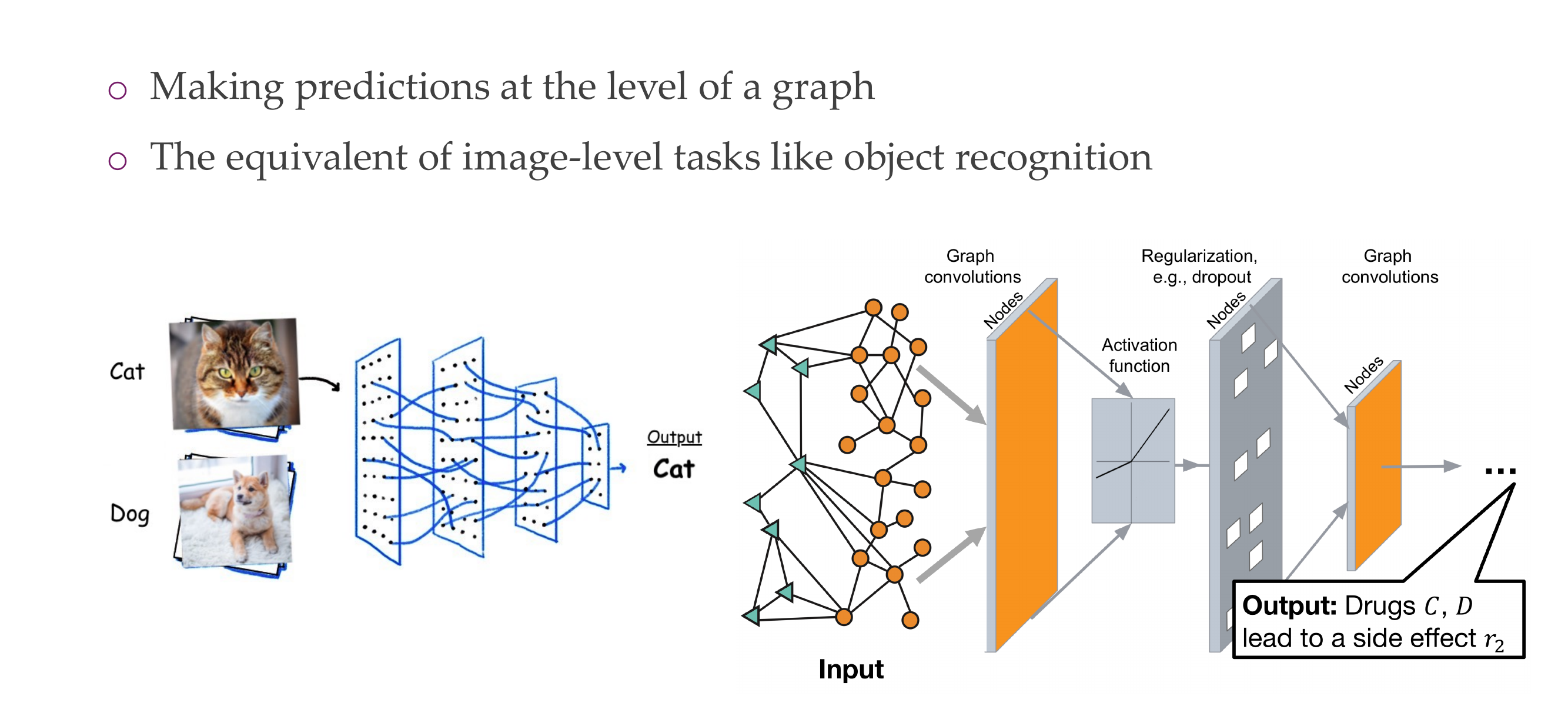
9 2) Classifying nodes

Slide 9

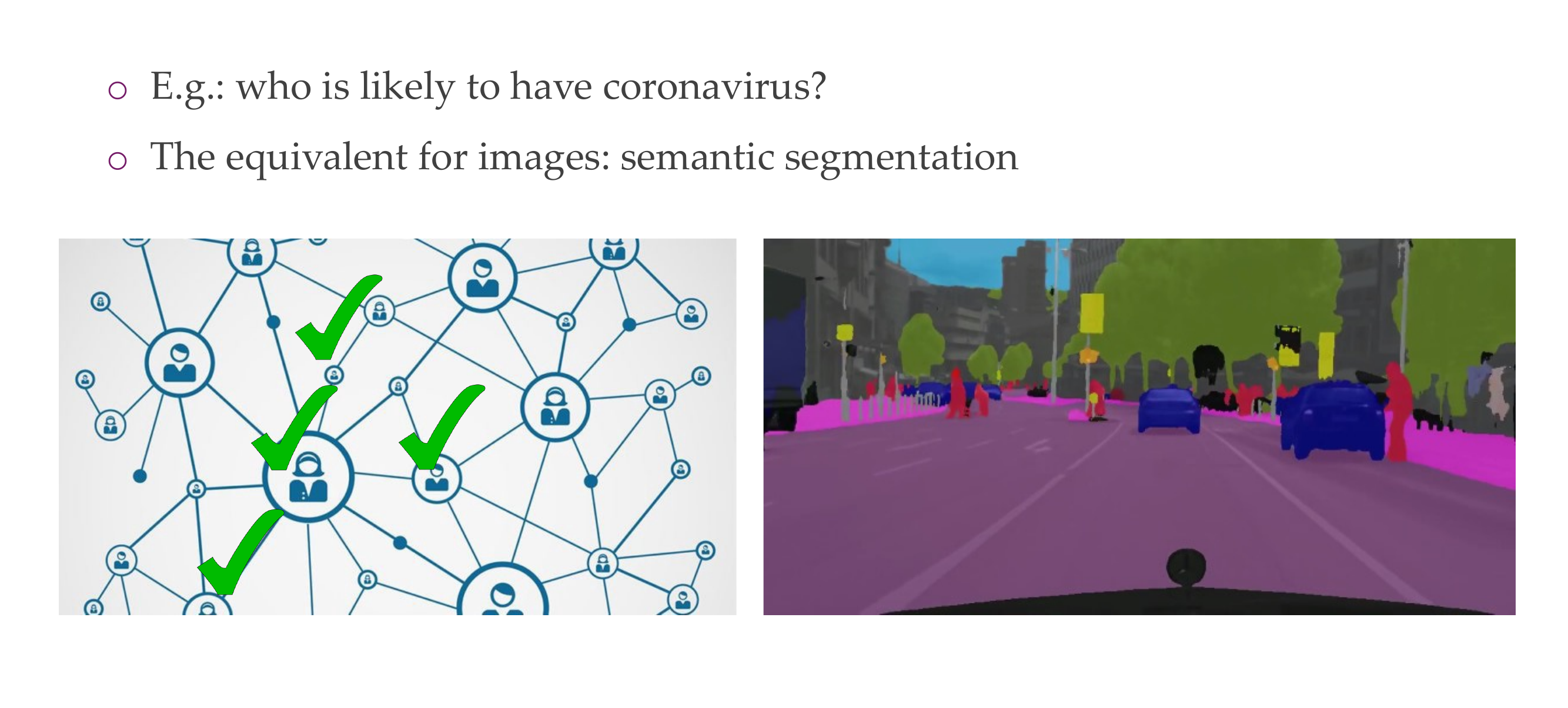
10 3) Graph generation

Slide 10

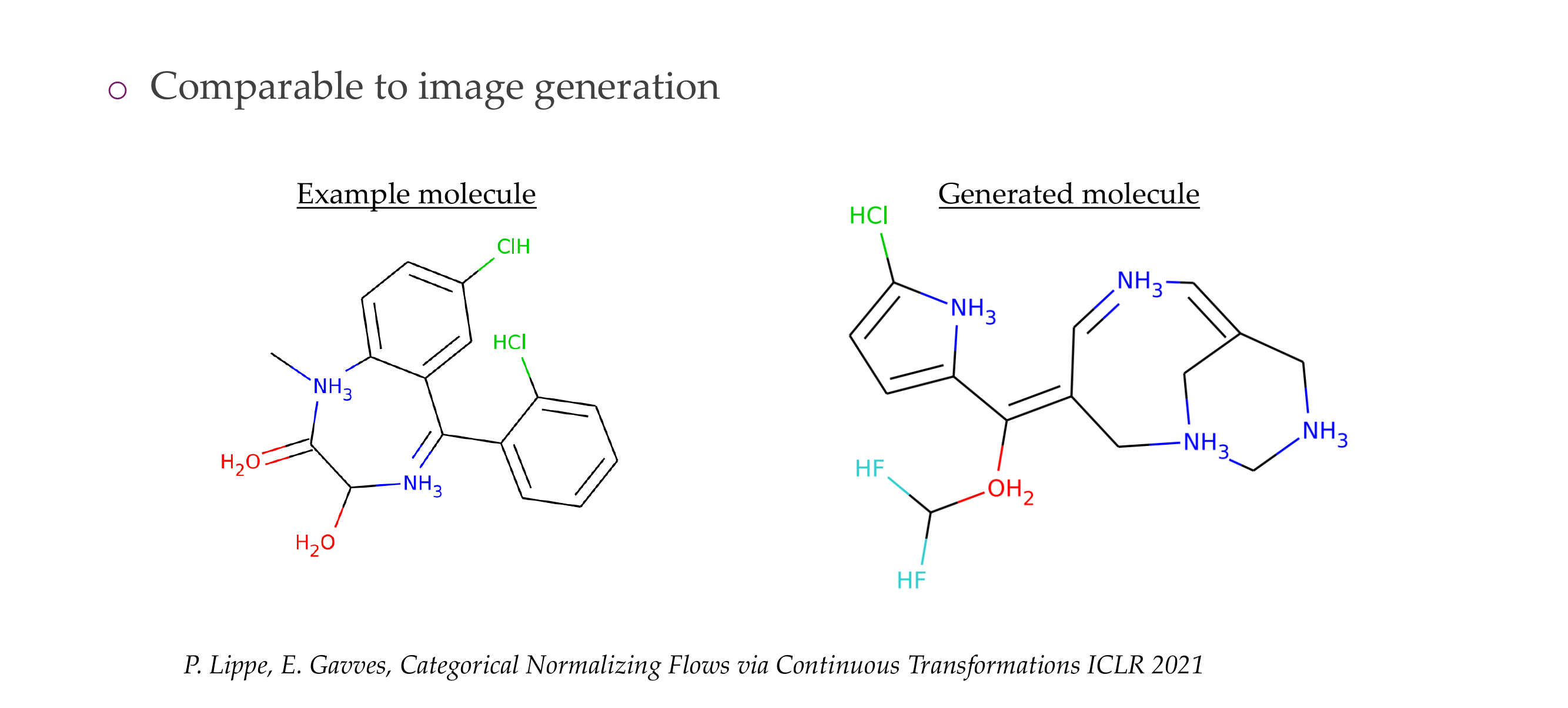
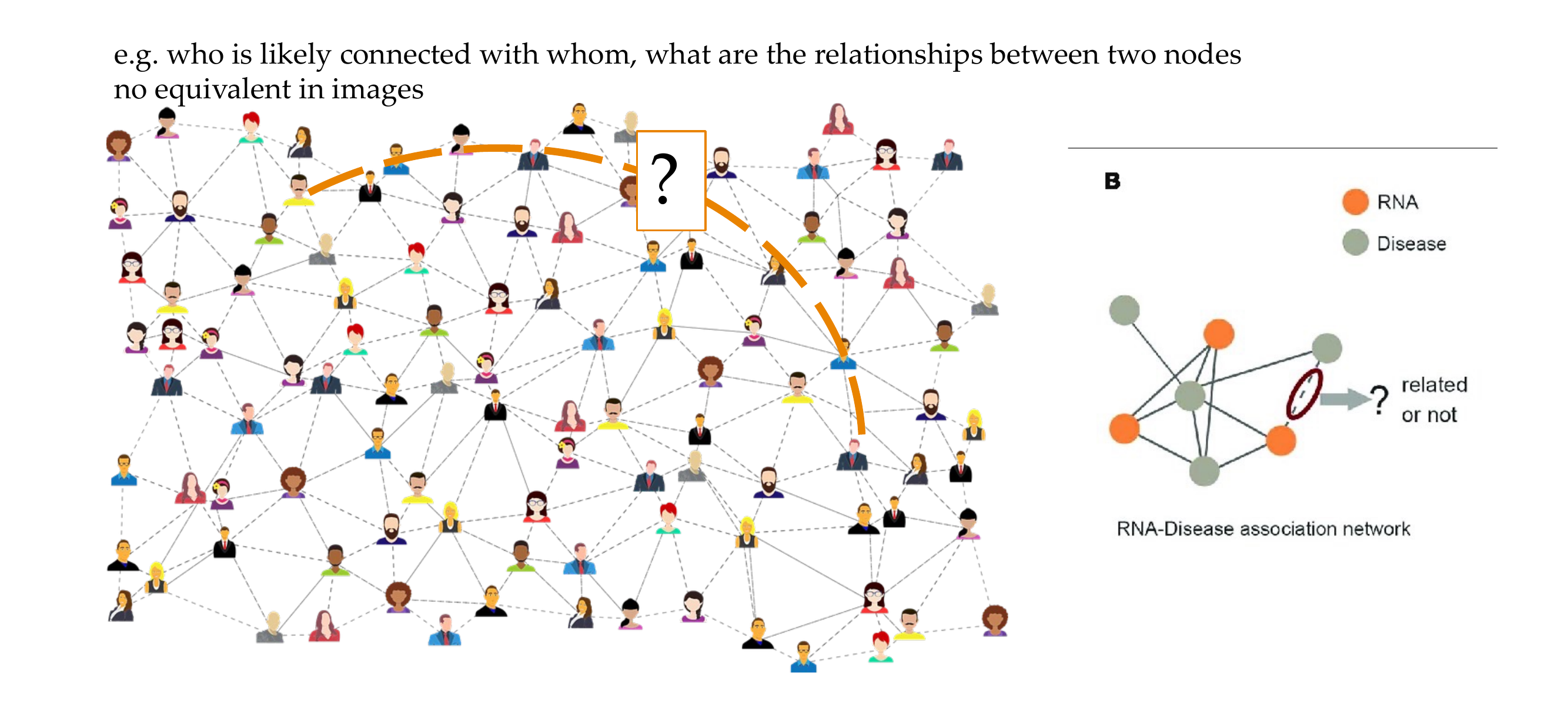
11 4) Link/Edge prediction

Slide 11

12 Three tasks visualized: here with nodes that carry features

Slide 12

13 Graphs can be static, varying, or even evolving with time

Slide 13

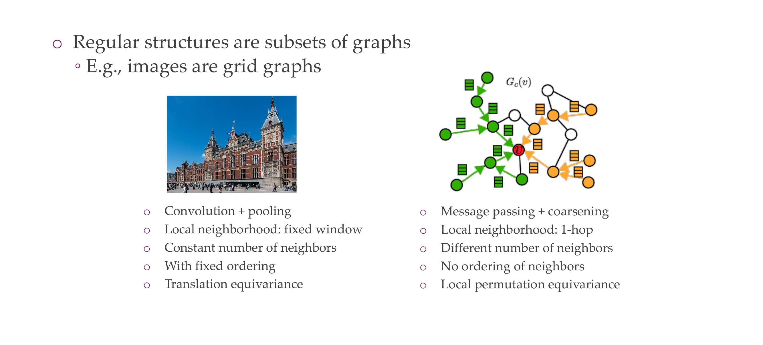
14 Regular structures vs graphs

Slide 14

15 Title

Slide 15

16 Directed graphs

Slide 16

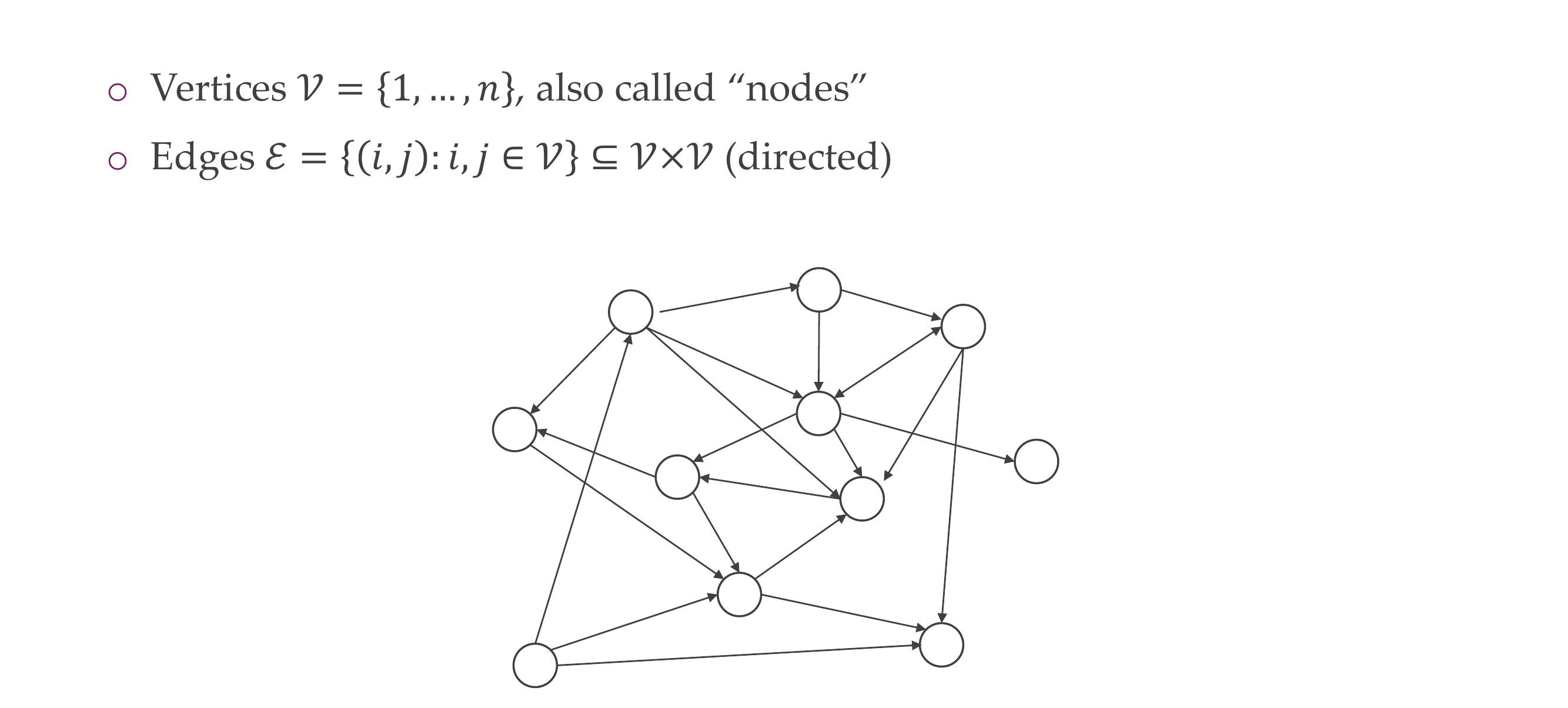
17 Undirected graphs

Slide 17

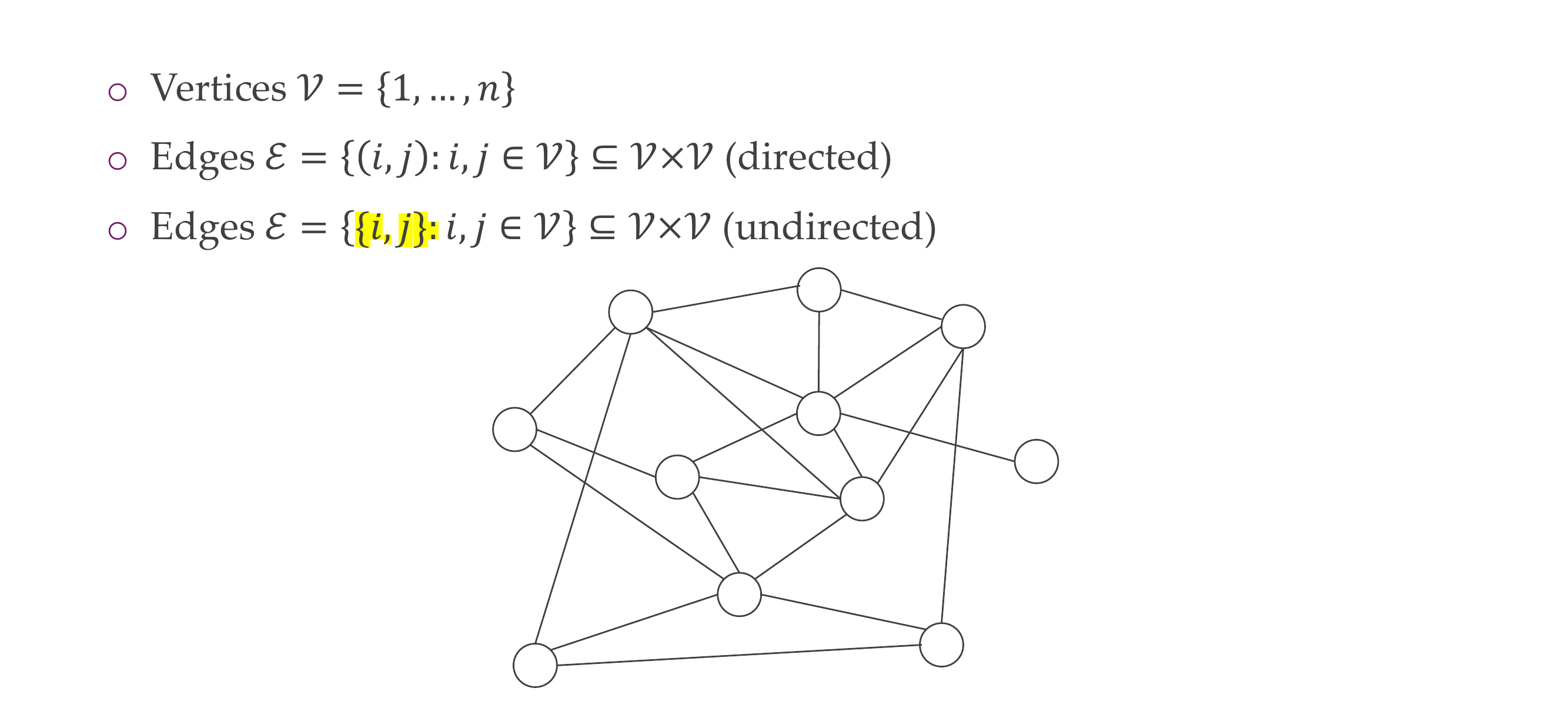
18 Graph neighborhood

Slide 18

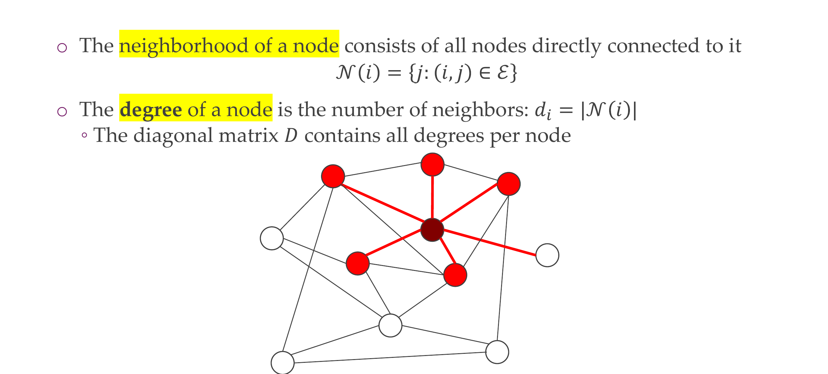
19 Attributes

Slide 19

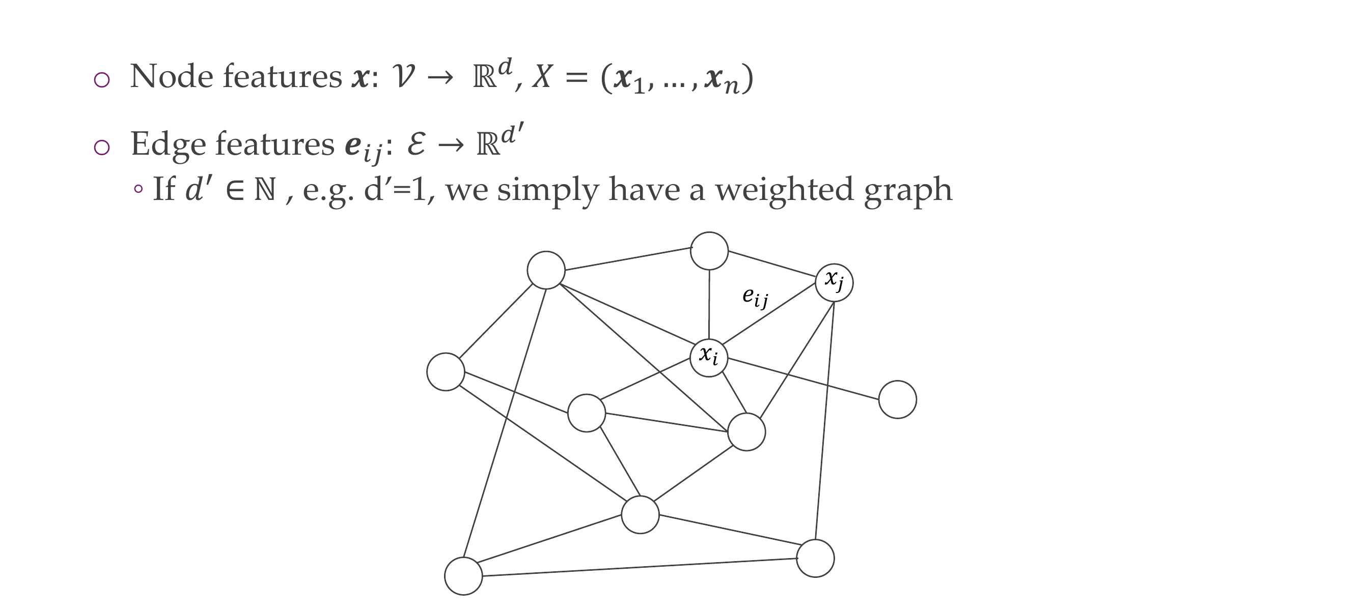
The attention score is measured by these softmax

The dot product here it ends up being 2x3 again

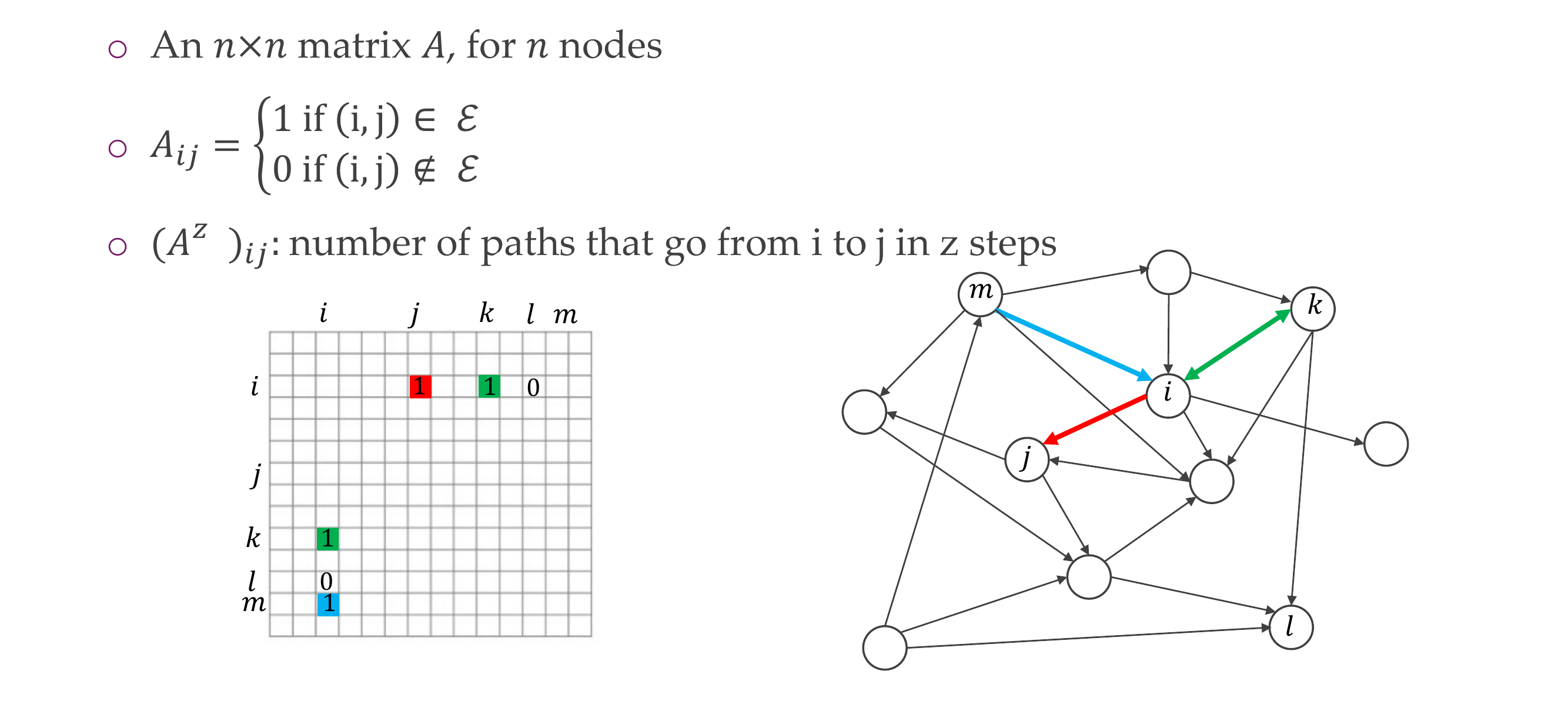
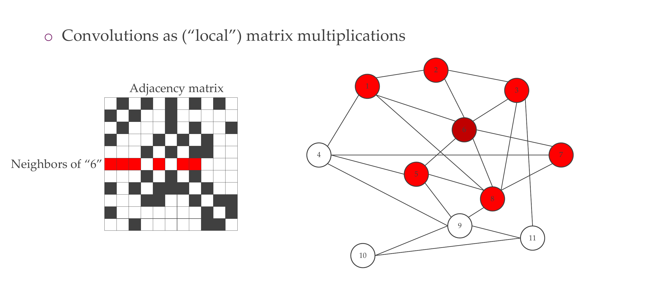
20 Adjacency matrix

Slide 20

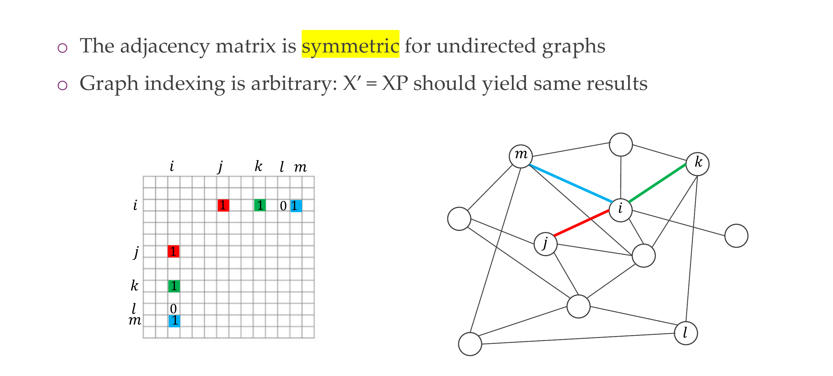
21 Adjacency matrix for undirected graphs

Slide 21

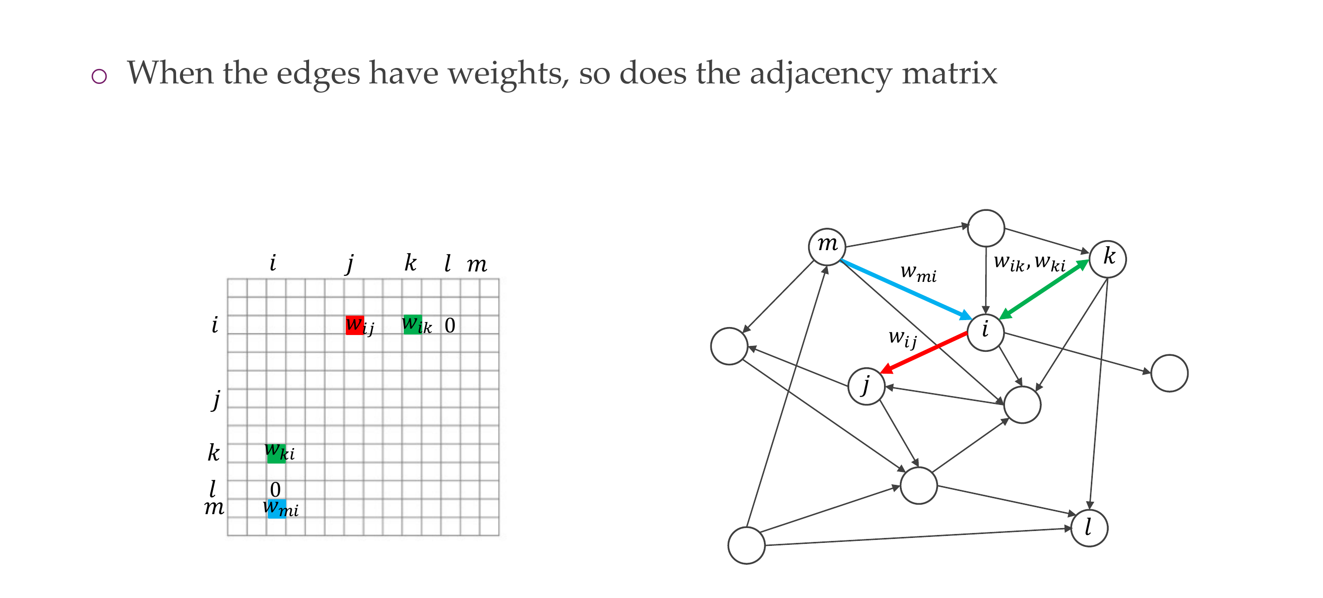
22 Weighted adjacency matrix

Slide 22

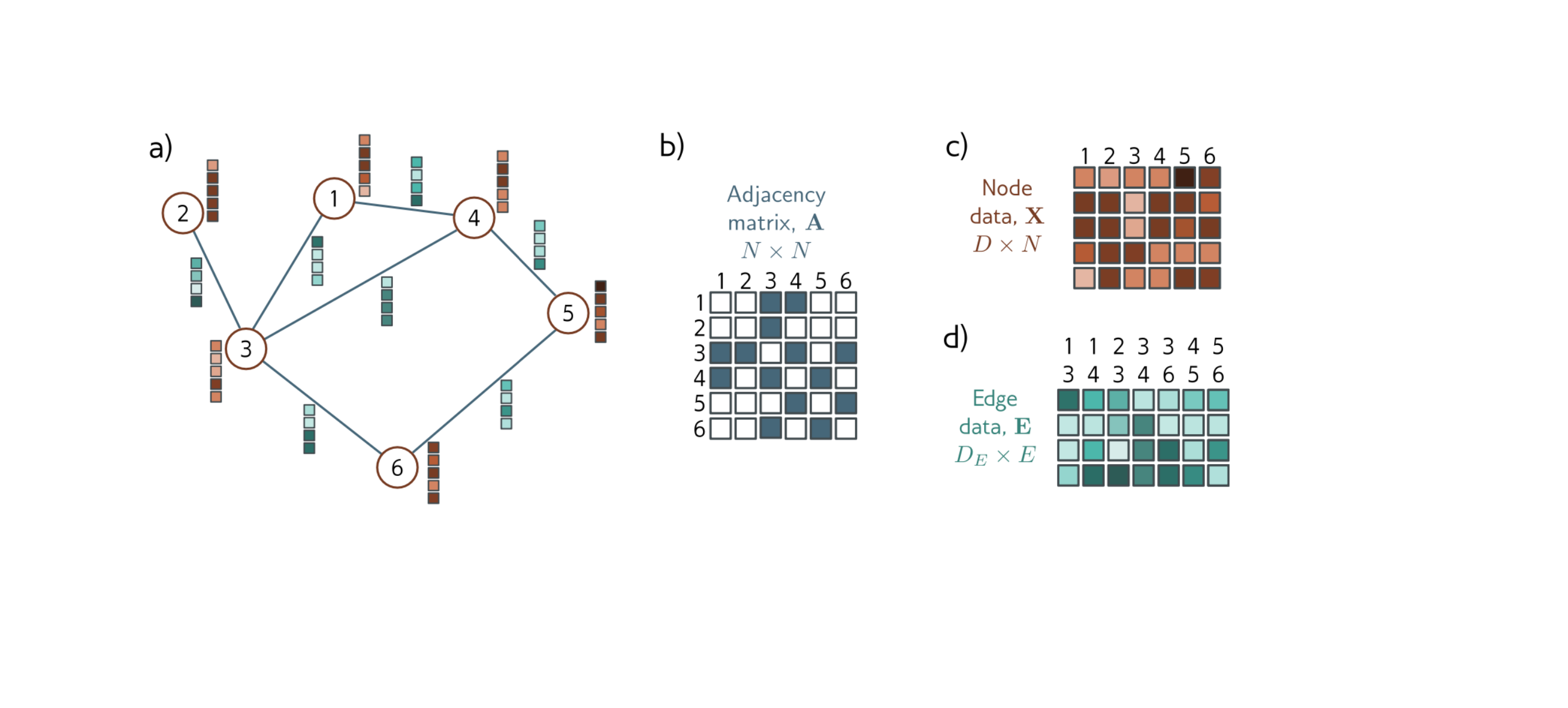
23 Graph representation for us

Slide 23

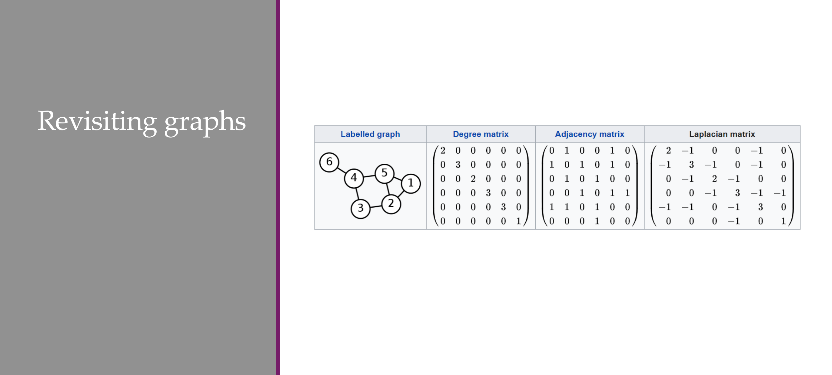
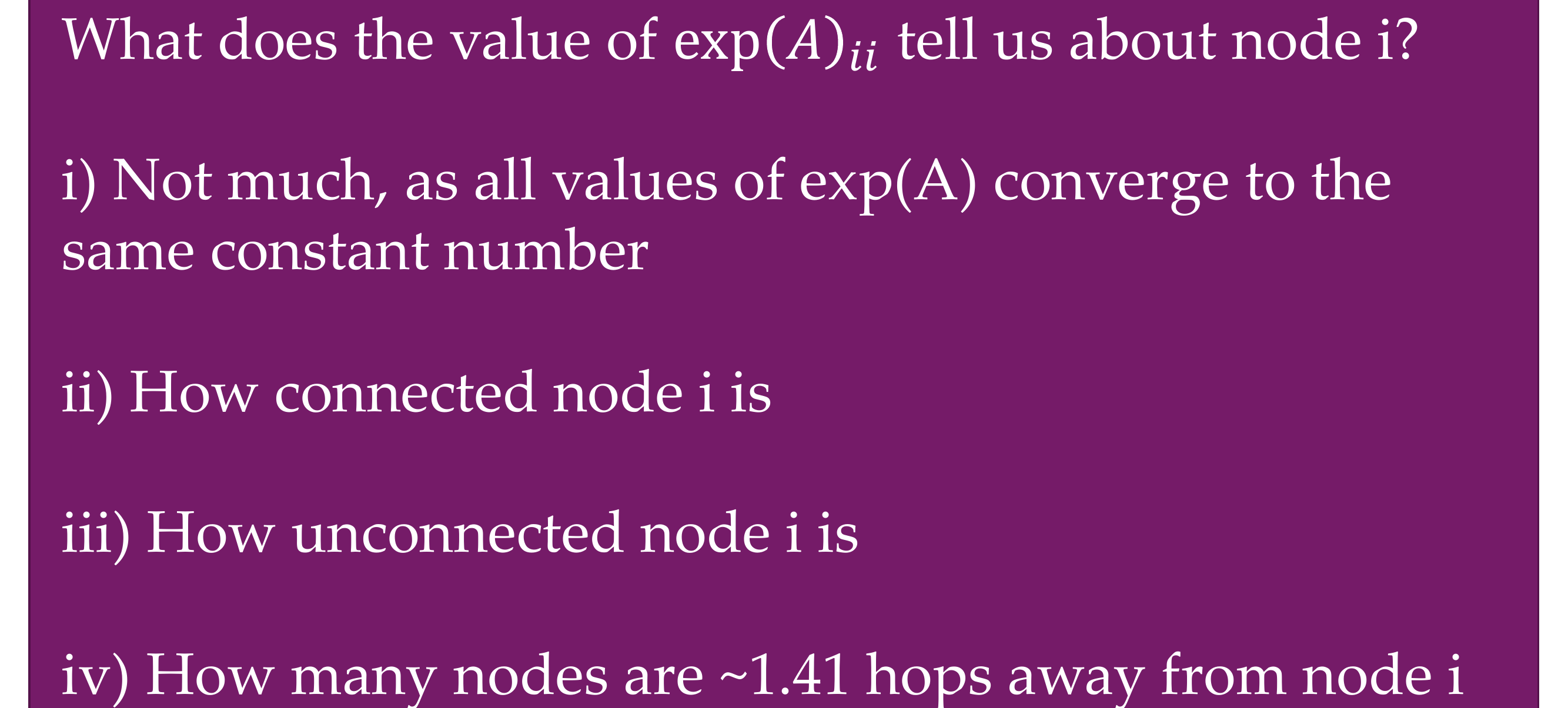
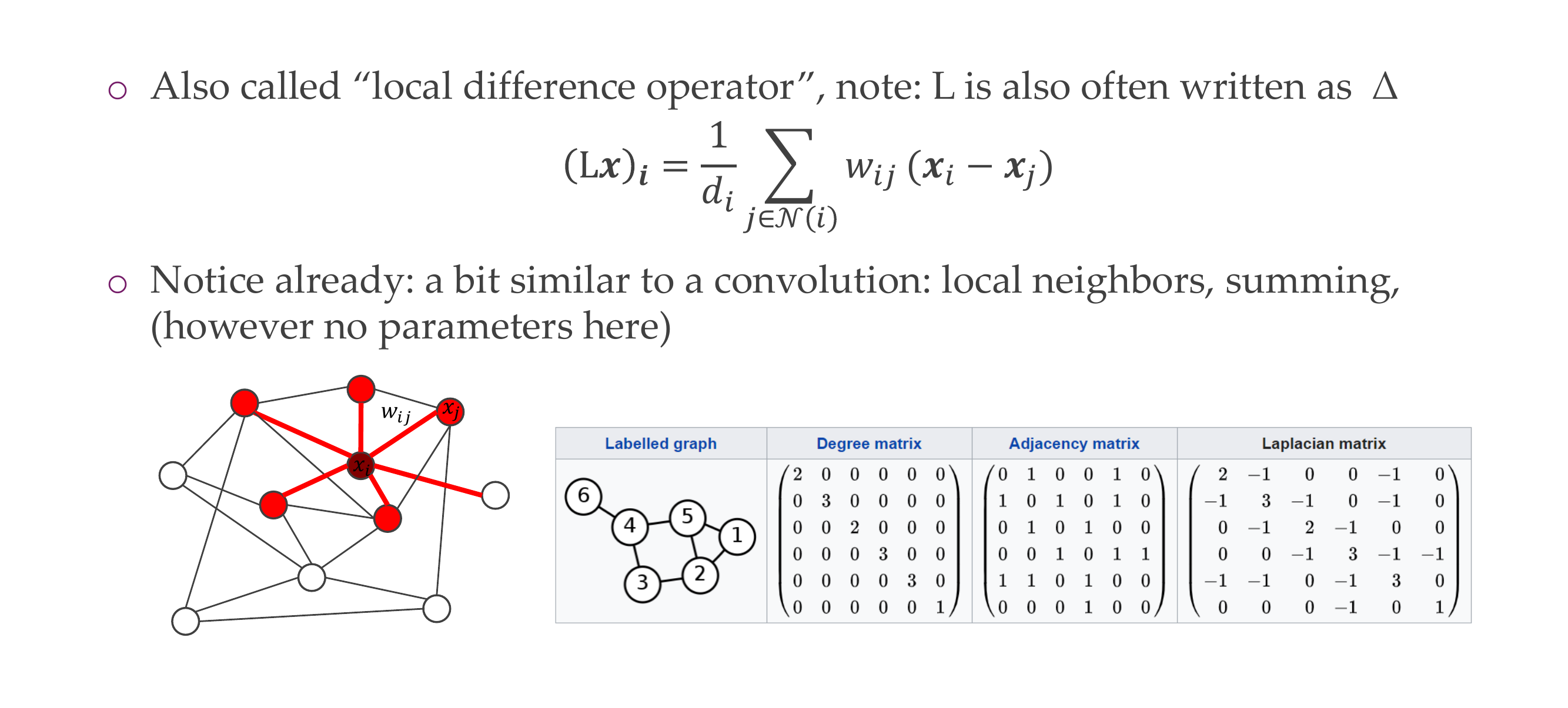
24 Quiz:

Slide 24

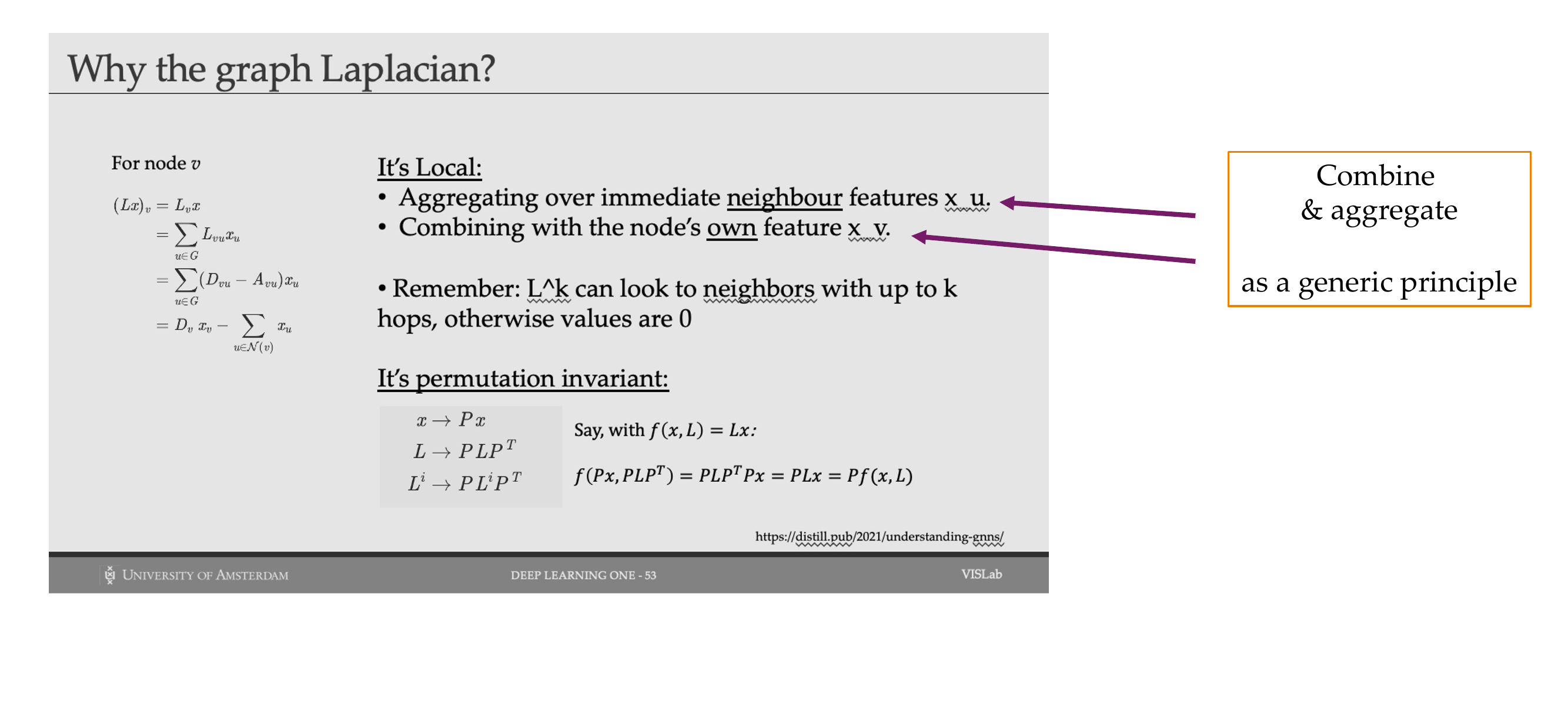
25 Graph Laplacian

Slide 25

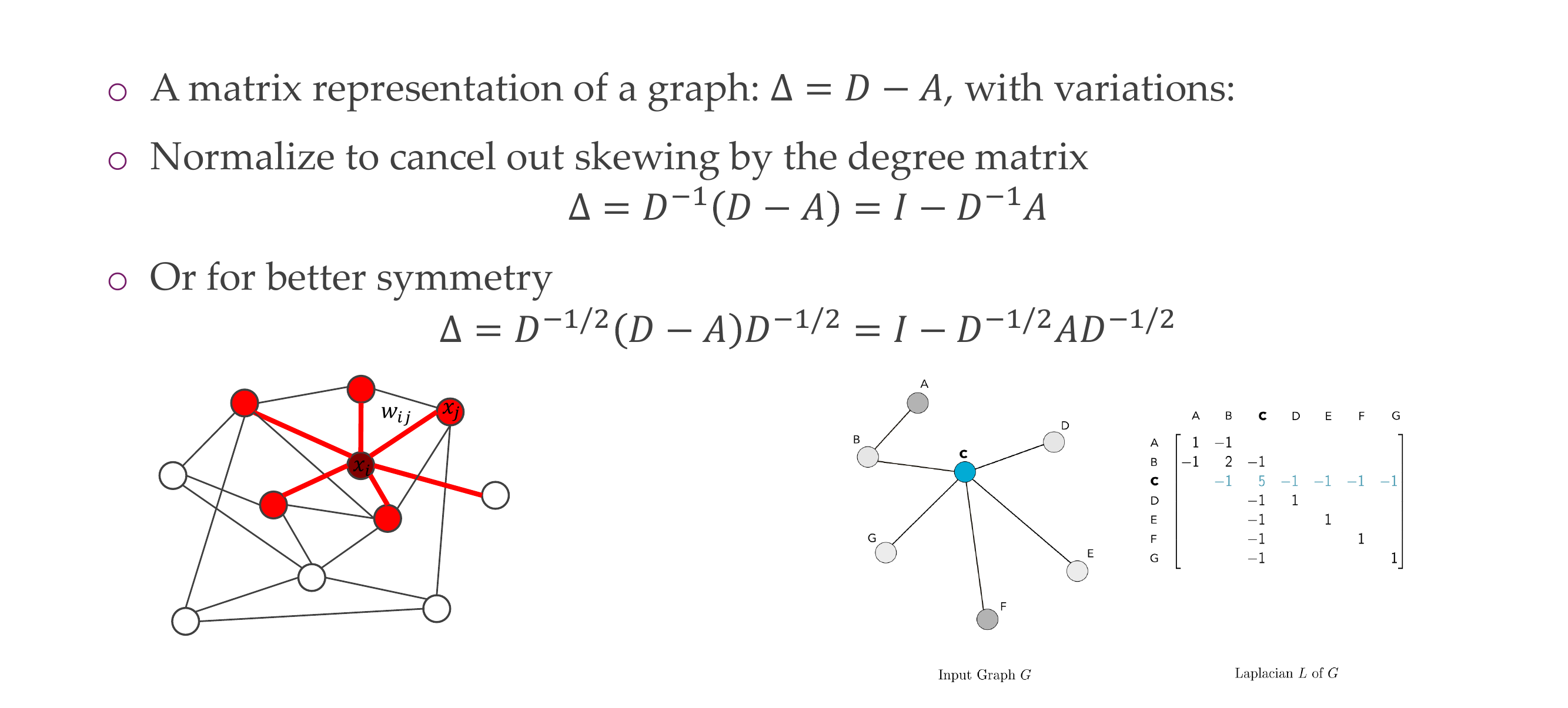
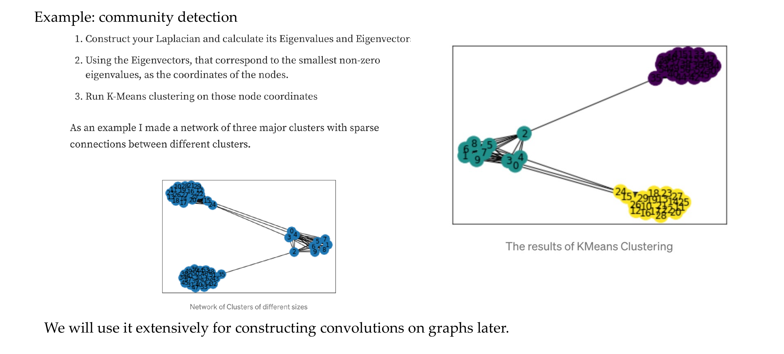
26 Graph Laplacian: meaning

Slide 26

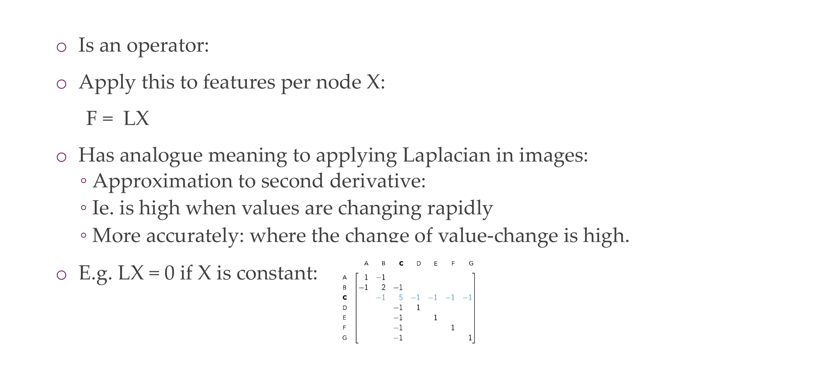
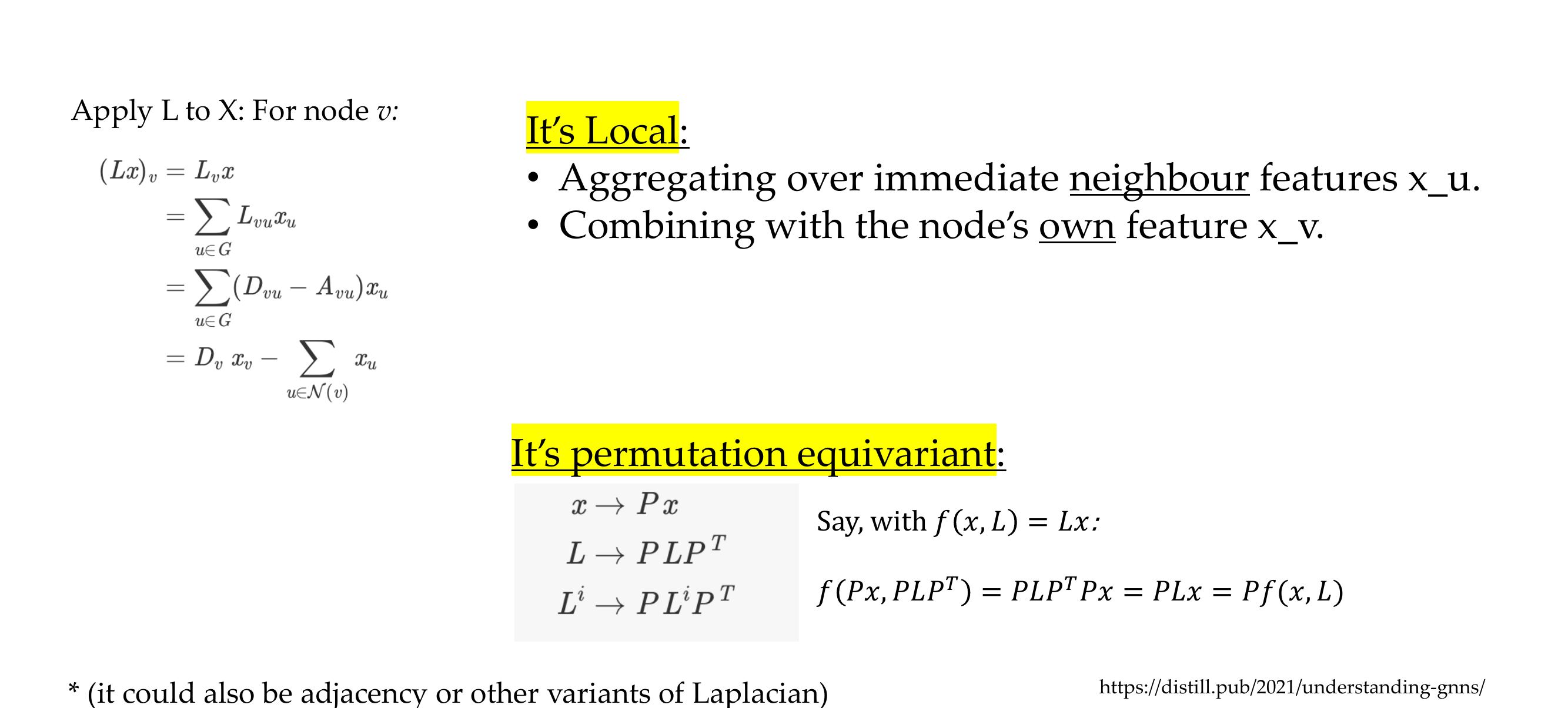
27 Applications of the Graph Laplacian

Slide 27

28 Applied Laplacian written out:

Slide 28

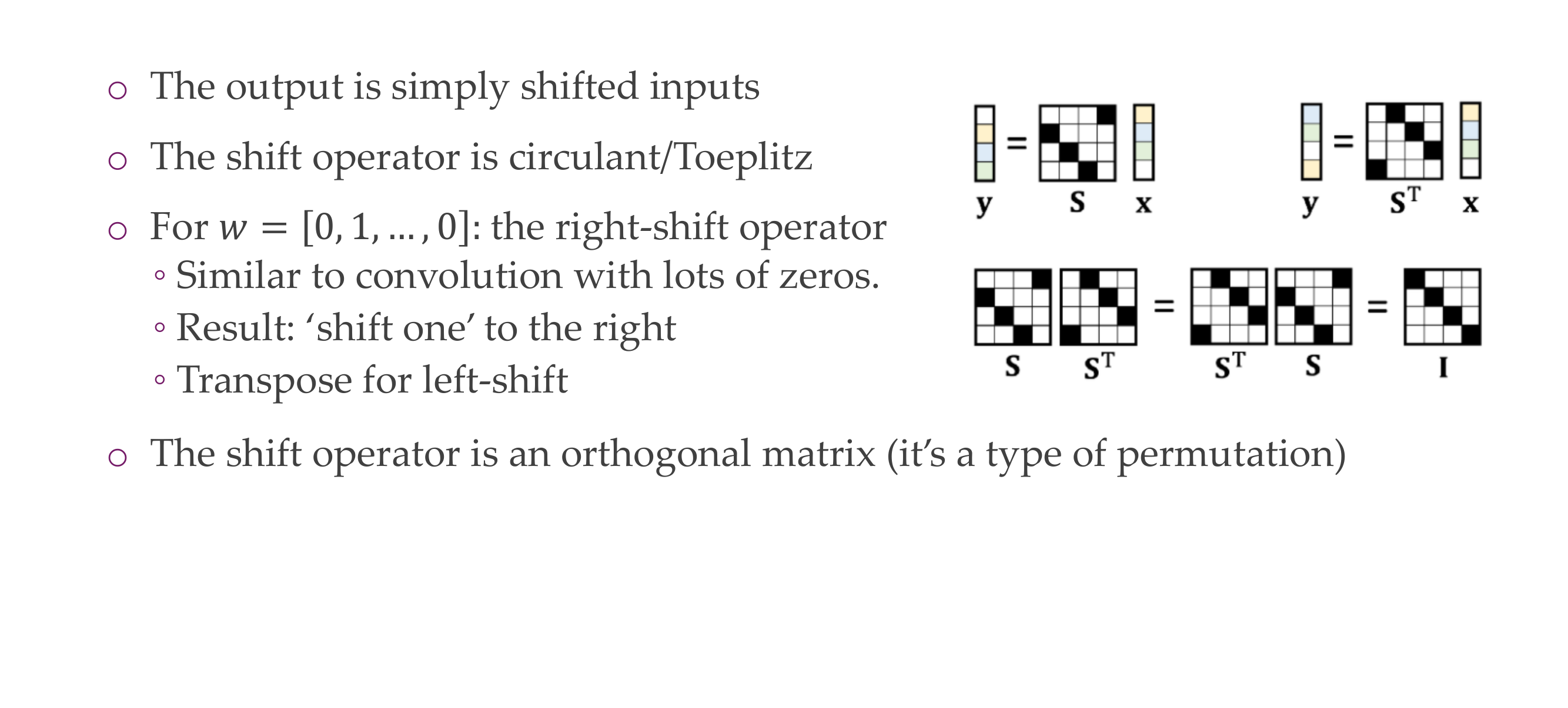
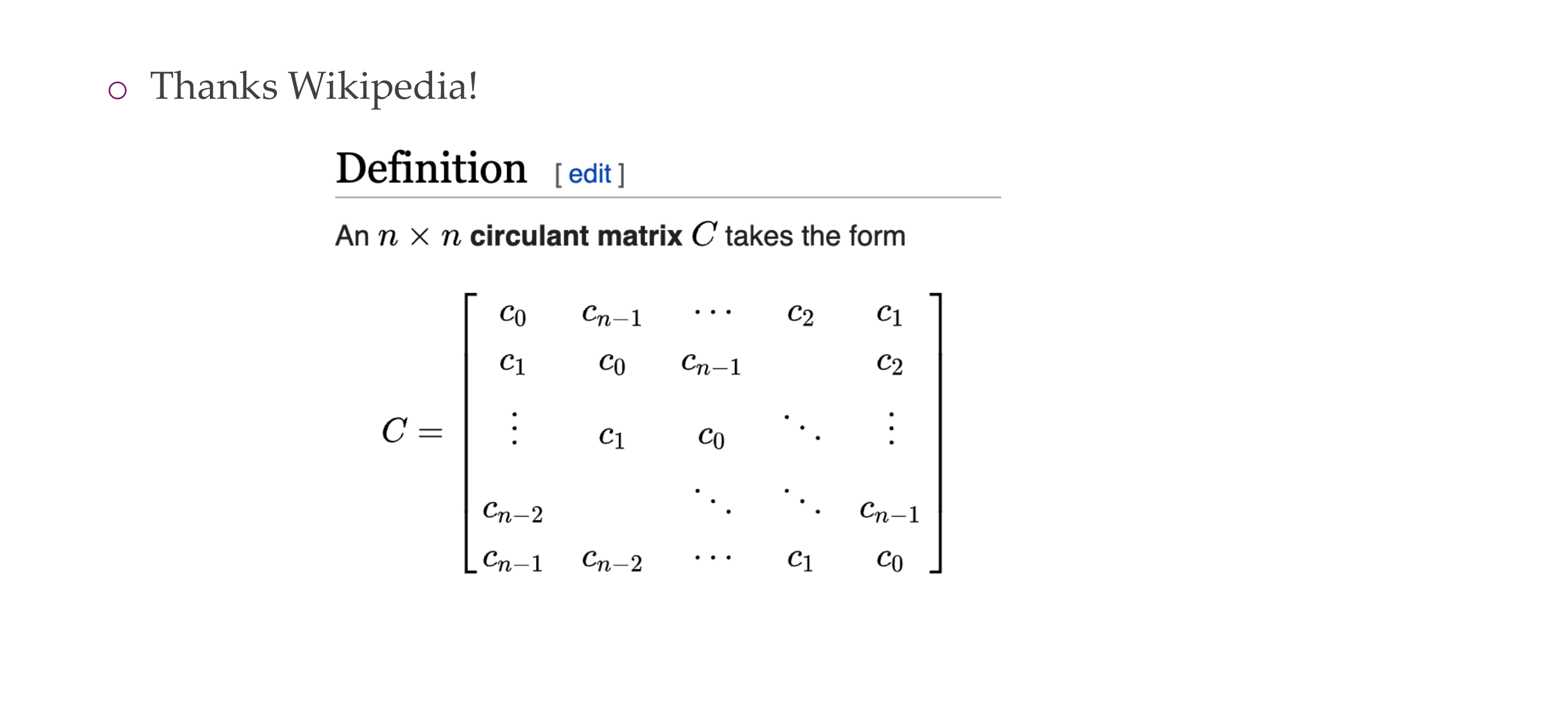
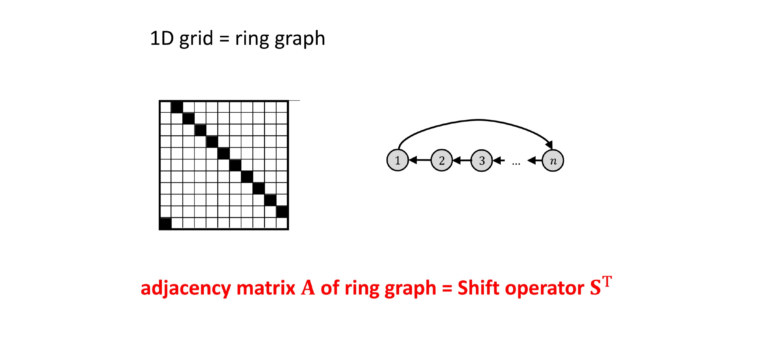
29 Title

Slide 29

30 The shift operator, a special circulant matrix

Slide 30

31 Now we want to know:

Slide 31

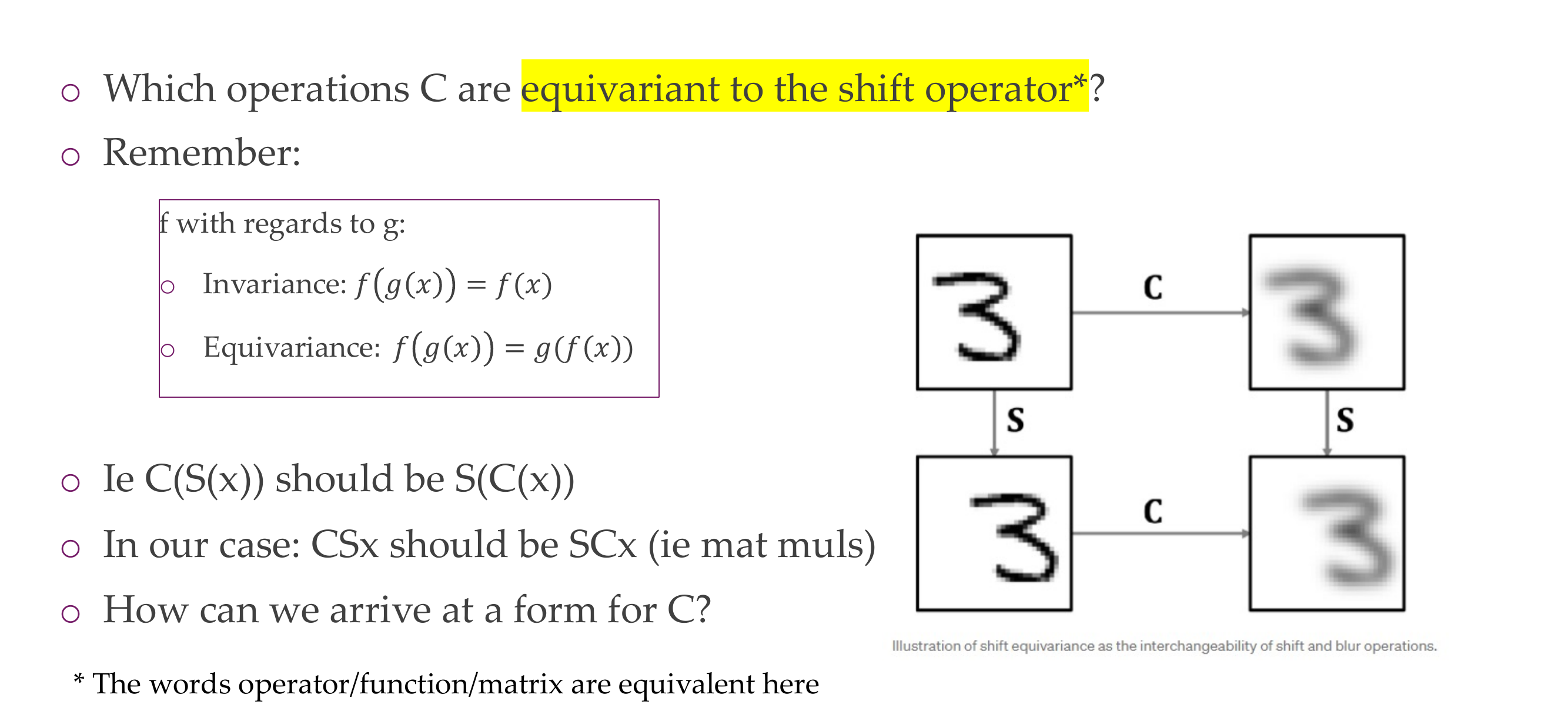
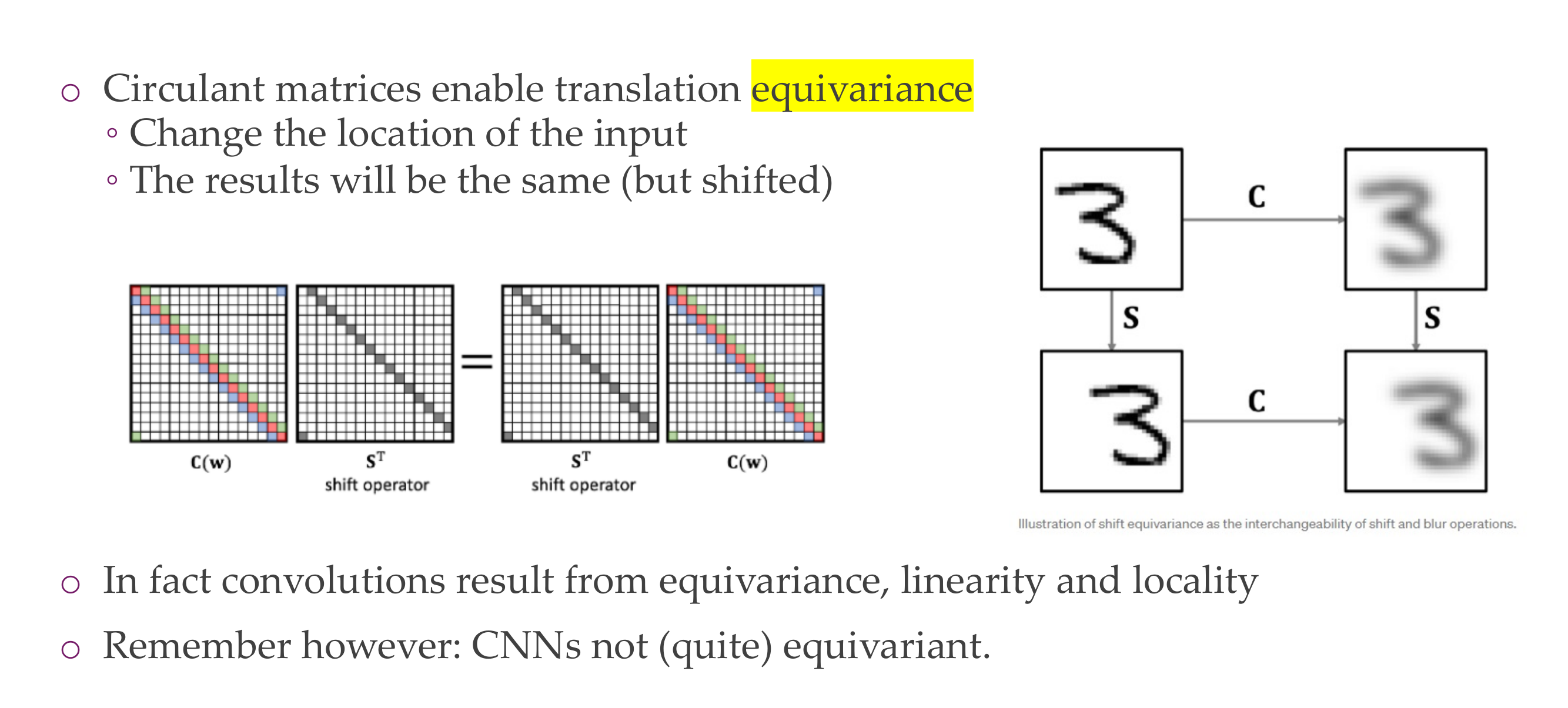
32 As it turns out: circulant matrices commute

Slide 32

33 What this means: Translation equivariance > circulant matrices/convolutions

Slide 33

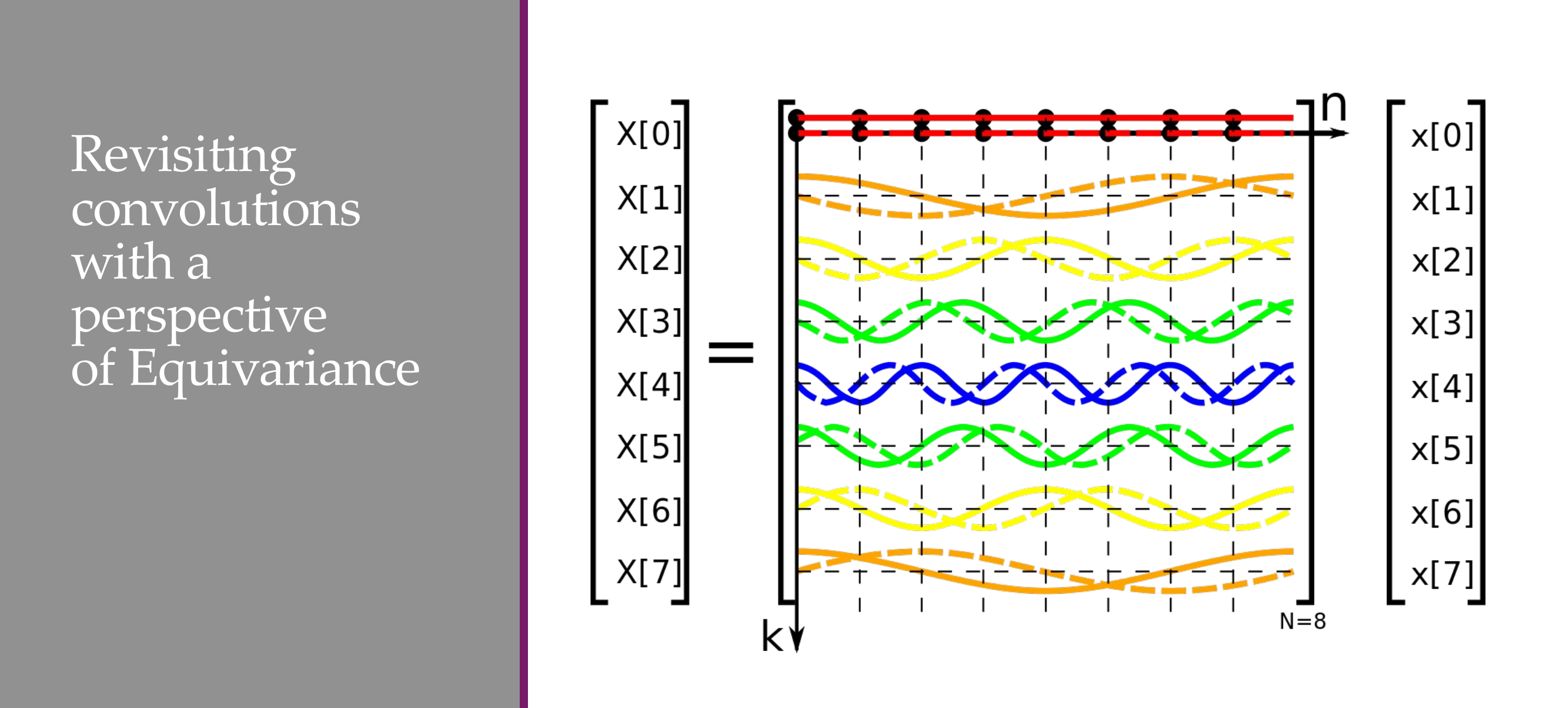
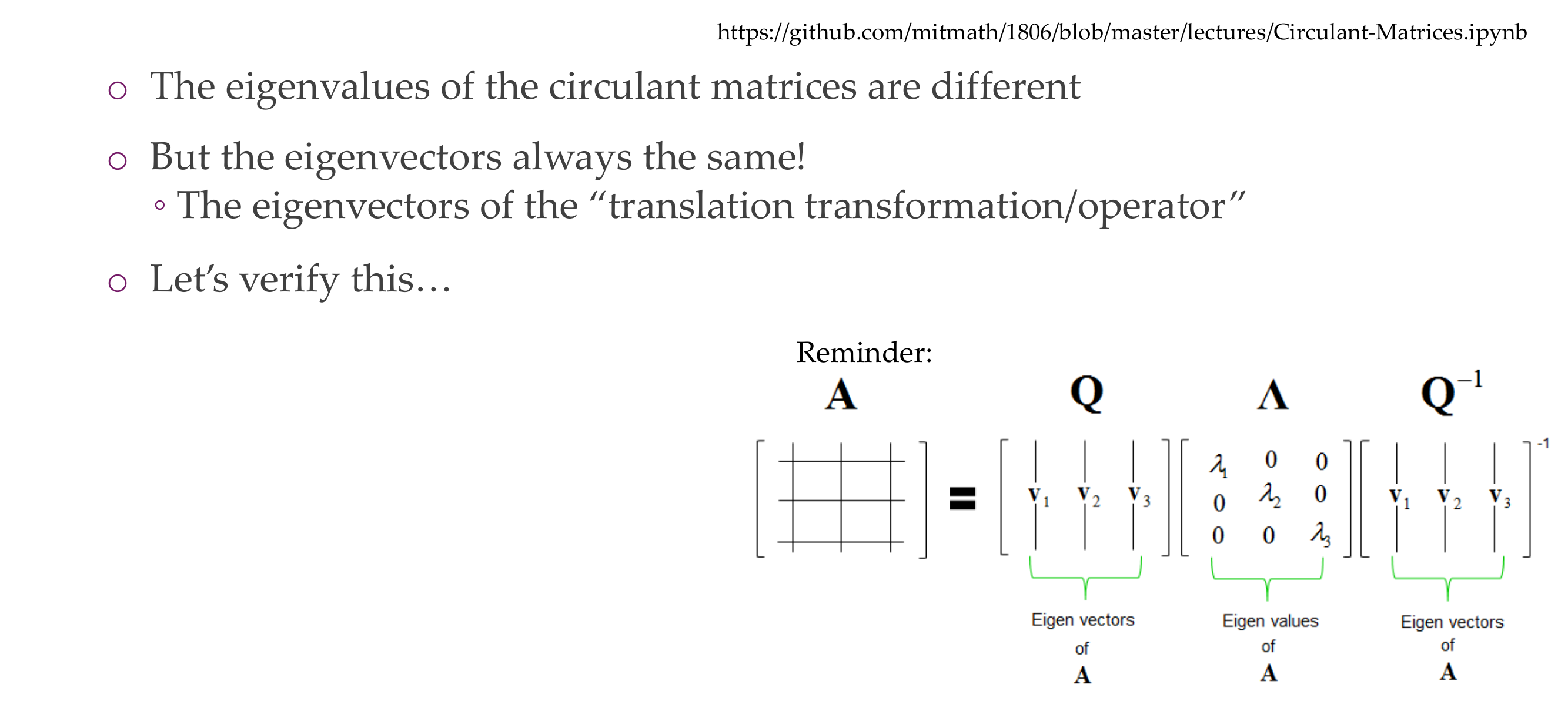
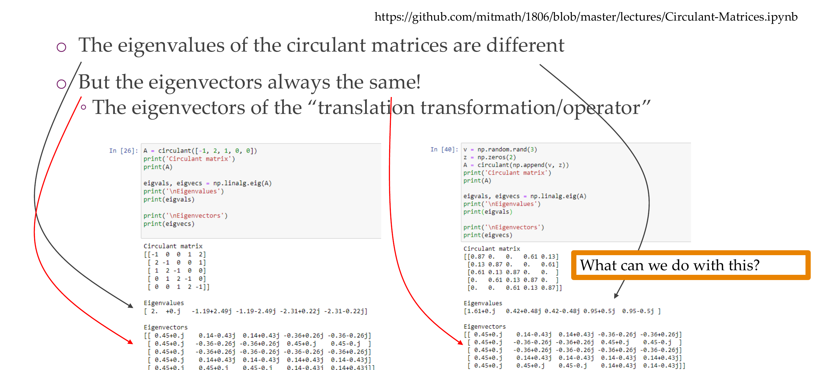
34 Where we are

Slide 34

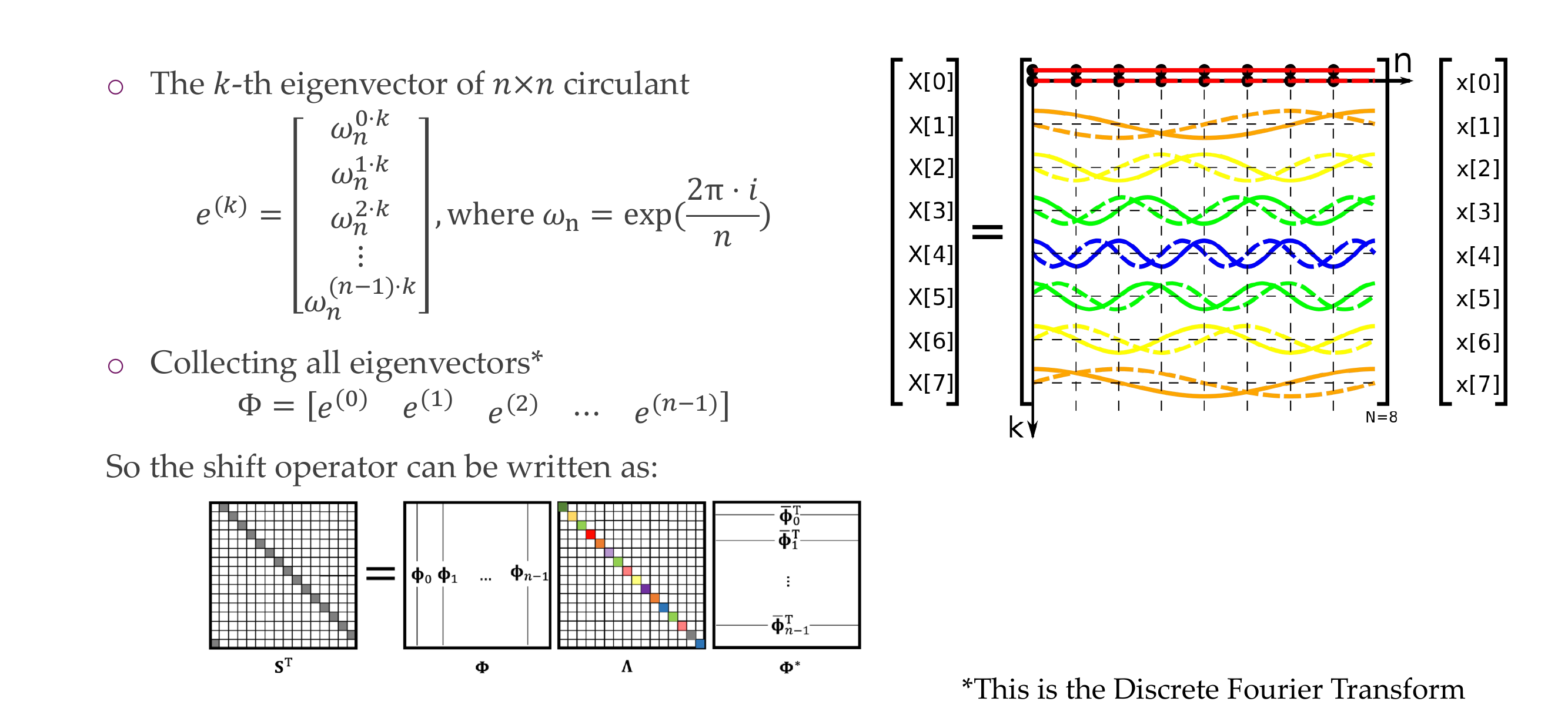
35 Maths: All circulant matrices have the same eigenvectors!

Slide 35

36 All circulant matrices have the same eigenvectors!

Slide 36

37 Circulant eigenvectors © Shift eigenvectors

Slide 37

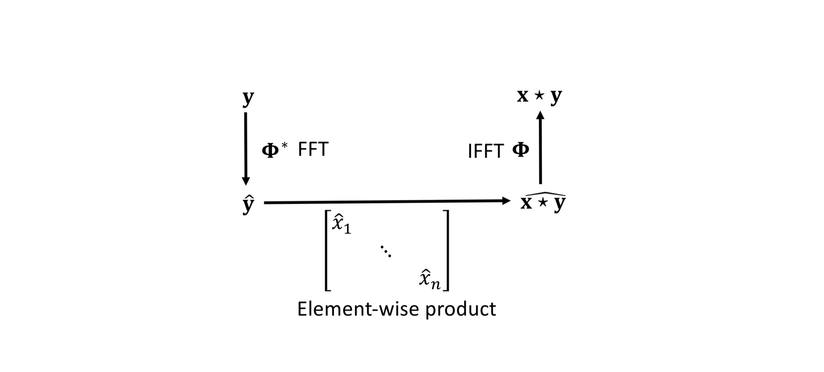
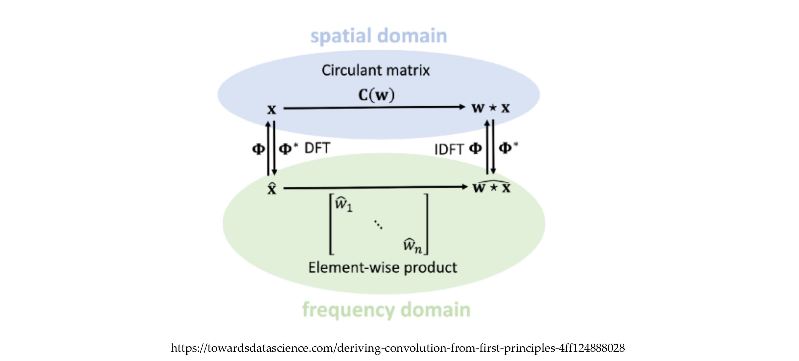
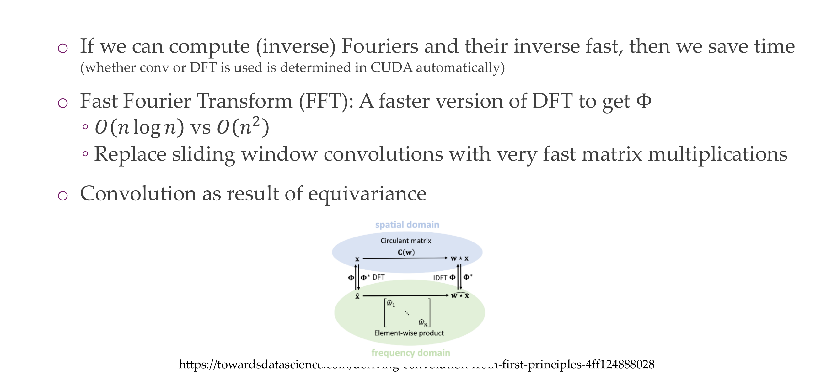
38 But first: What are the eigenvectors of the shift operator

Slide 38

39 Computing a convolution in the frequency domain

Slide 39

40 Convolution Theorem

Slide 40

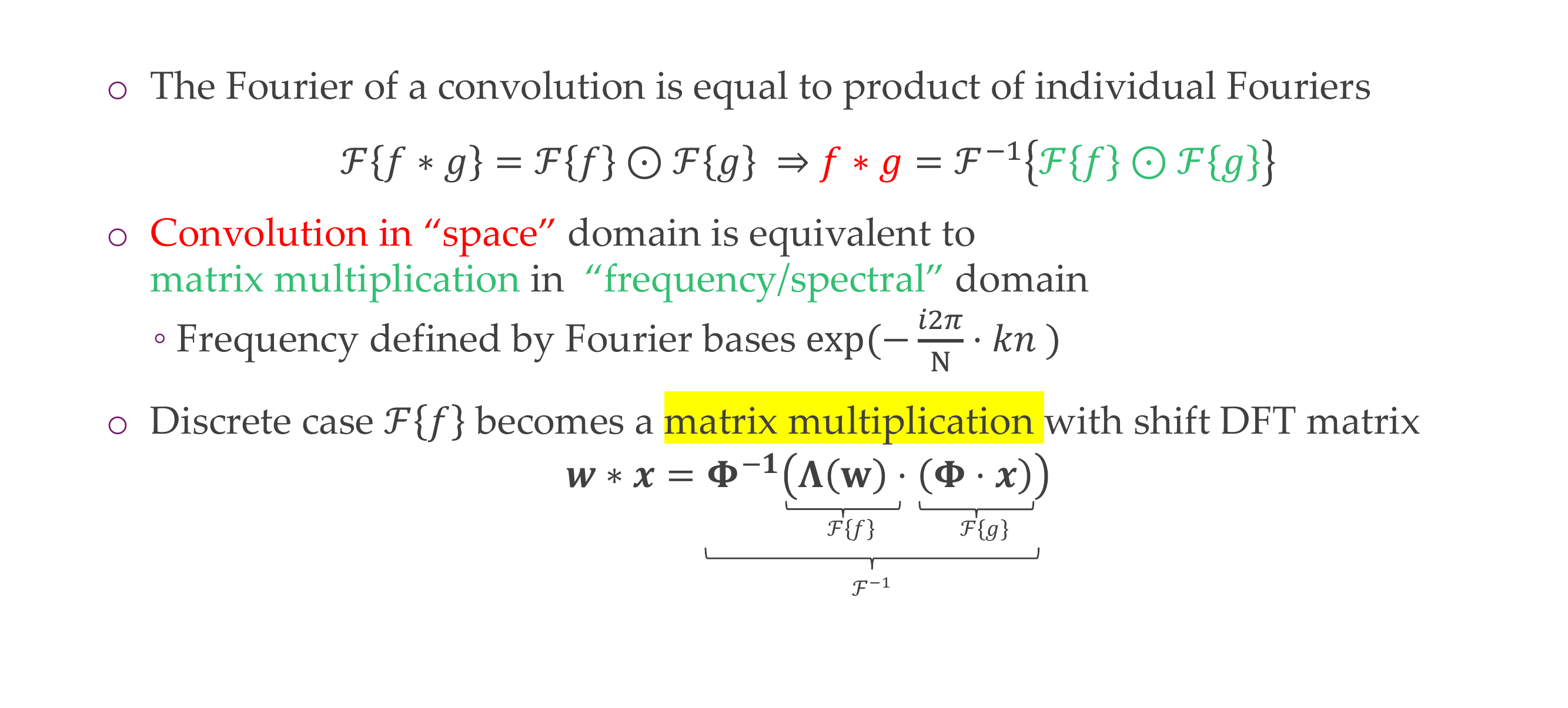
41 Convolution theorem

Slide 41

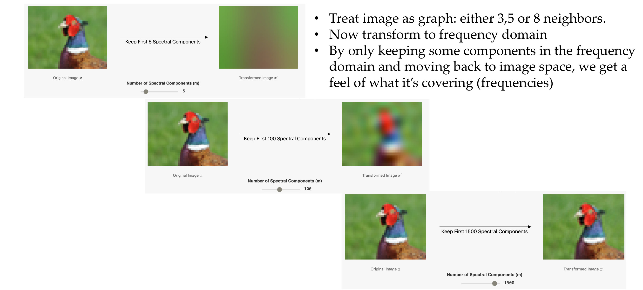
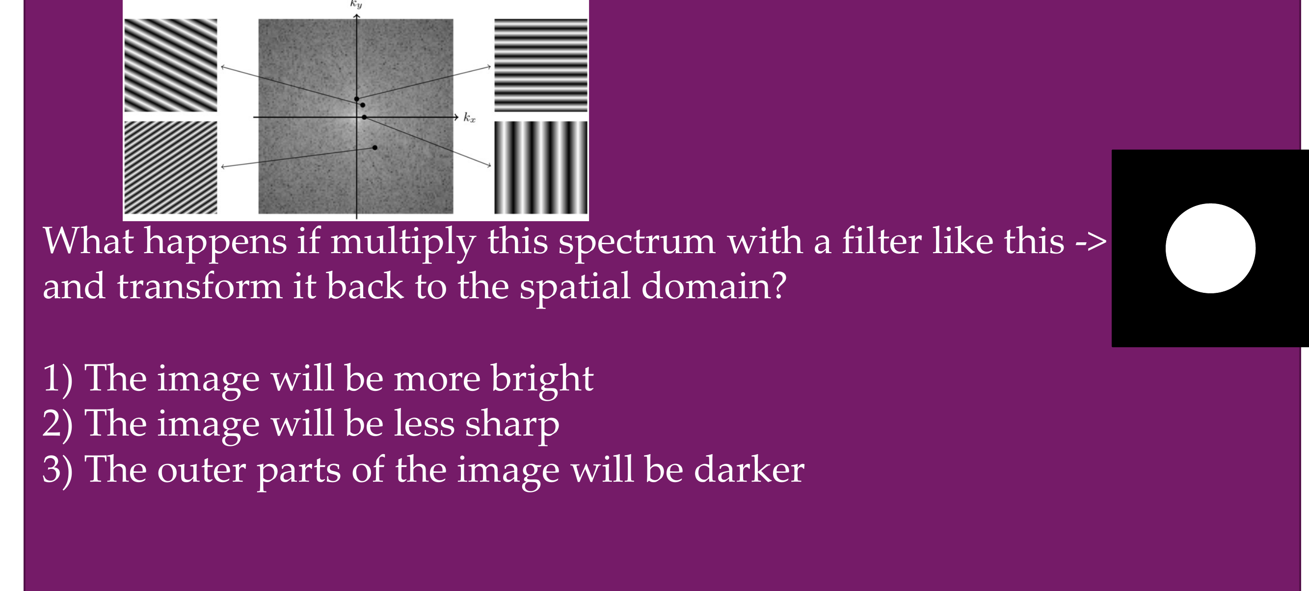
42 Frequency representation:

Slide 42

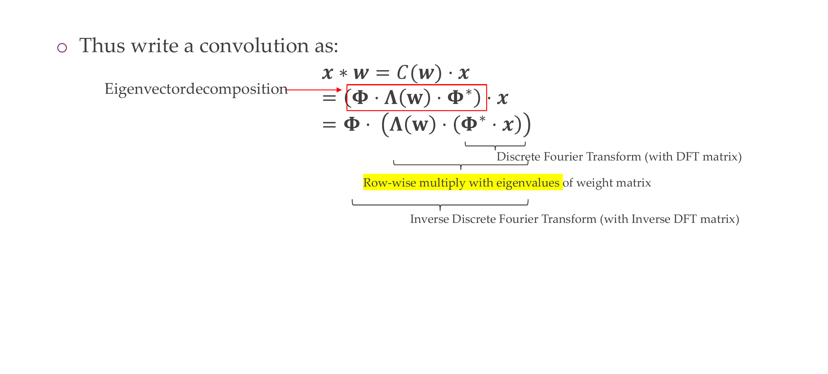
43 ; Quiz: Remember the Fourier transform for images: |

Slide 43

44 Convolution theorem: x * w = ®- (A(w) - (®* - x))

Slide 44

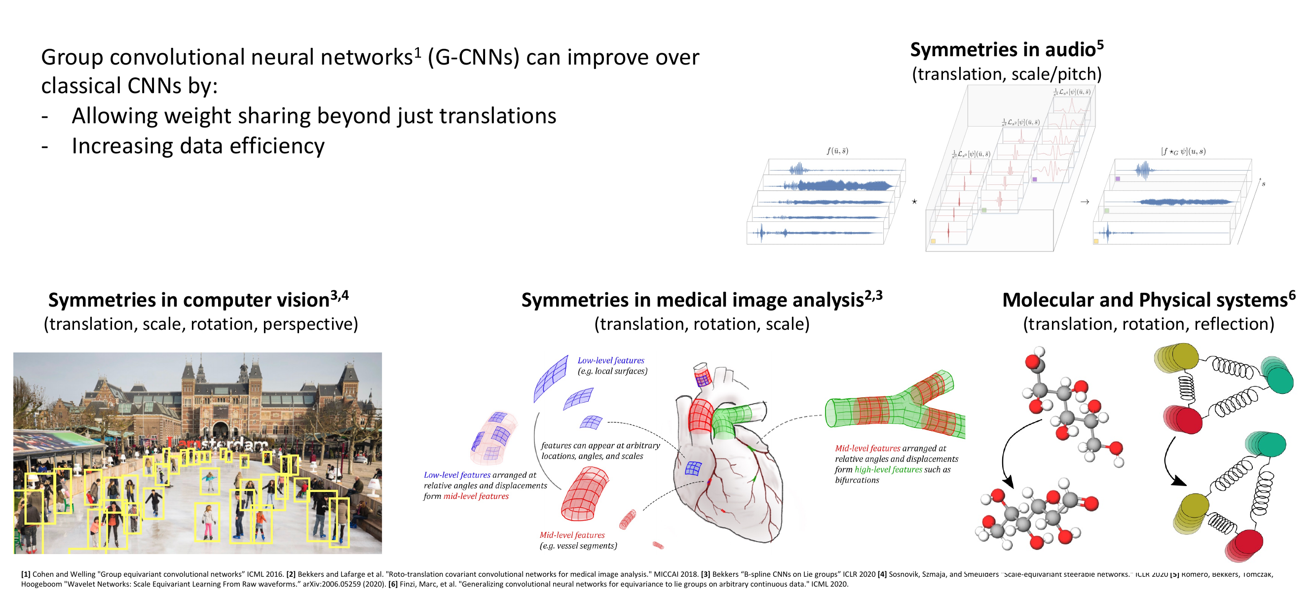
45 Implications

Slide 45

46 If translation equivariance leads to CNNs, what else is there?

Slide 46

47 A large field: Group Equivariant Deep Learning

Slide 47

48 Circulant matrices

Slide 48

49 “I was lucky…

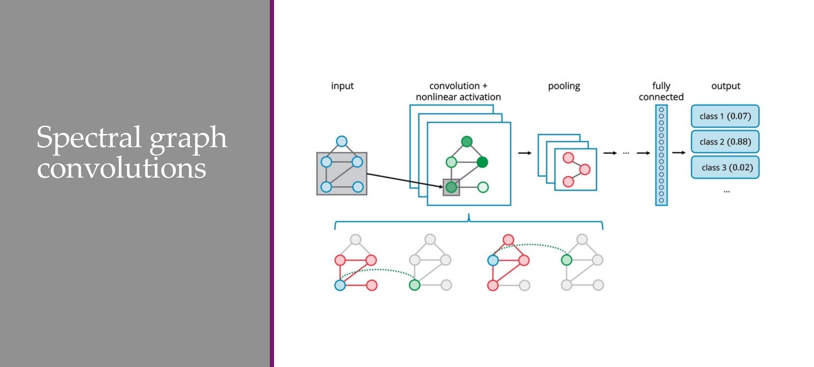
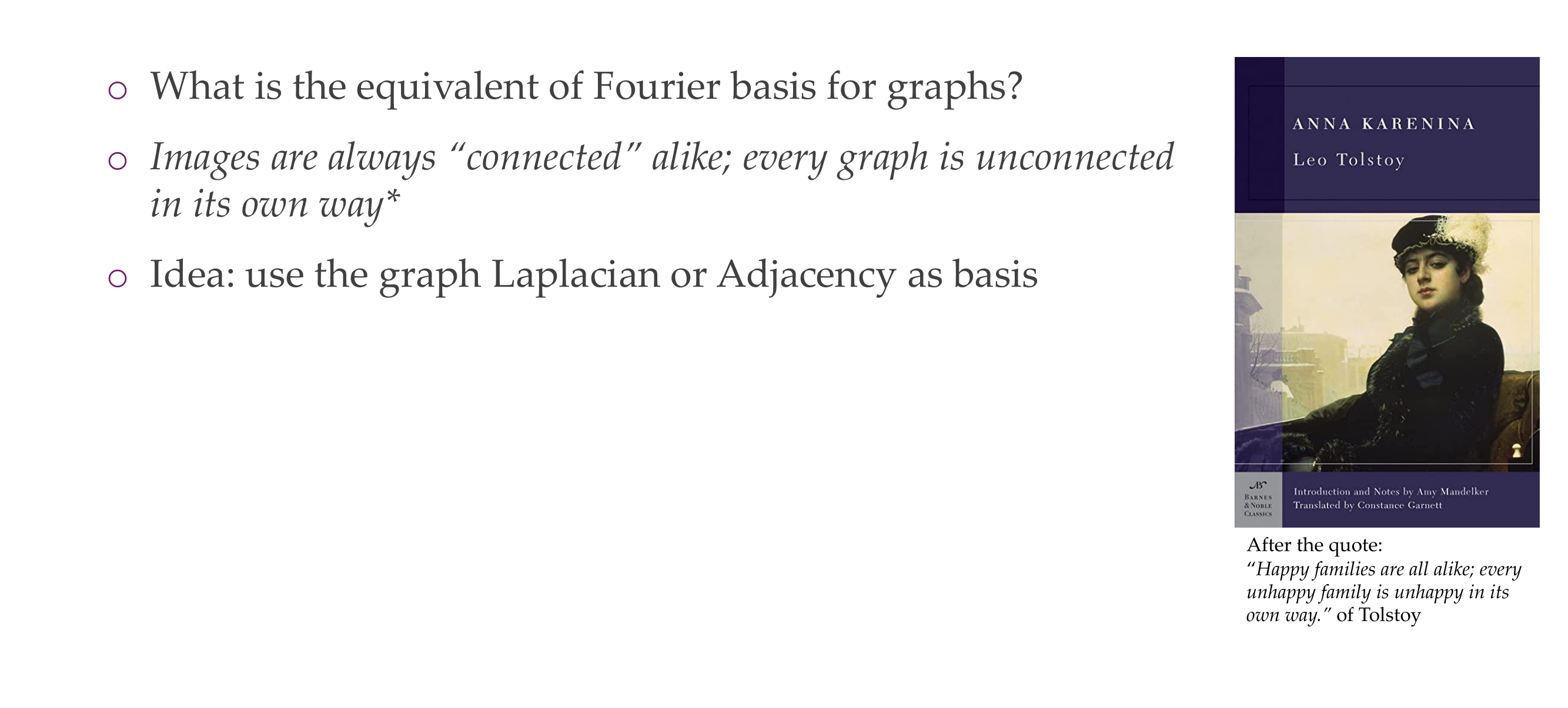
How research gets done part 6

Slide 49

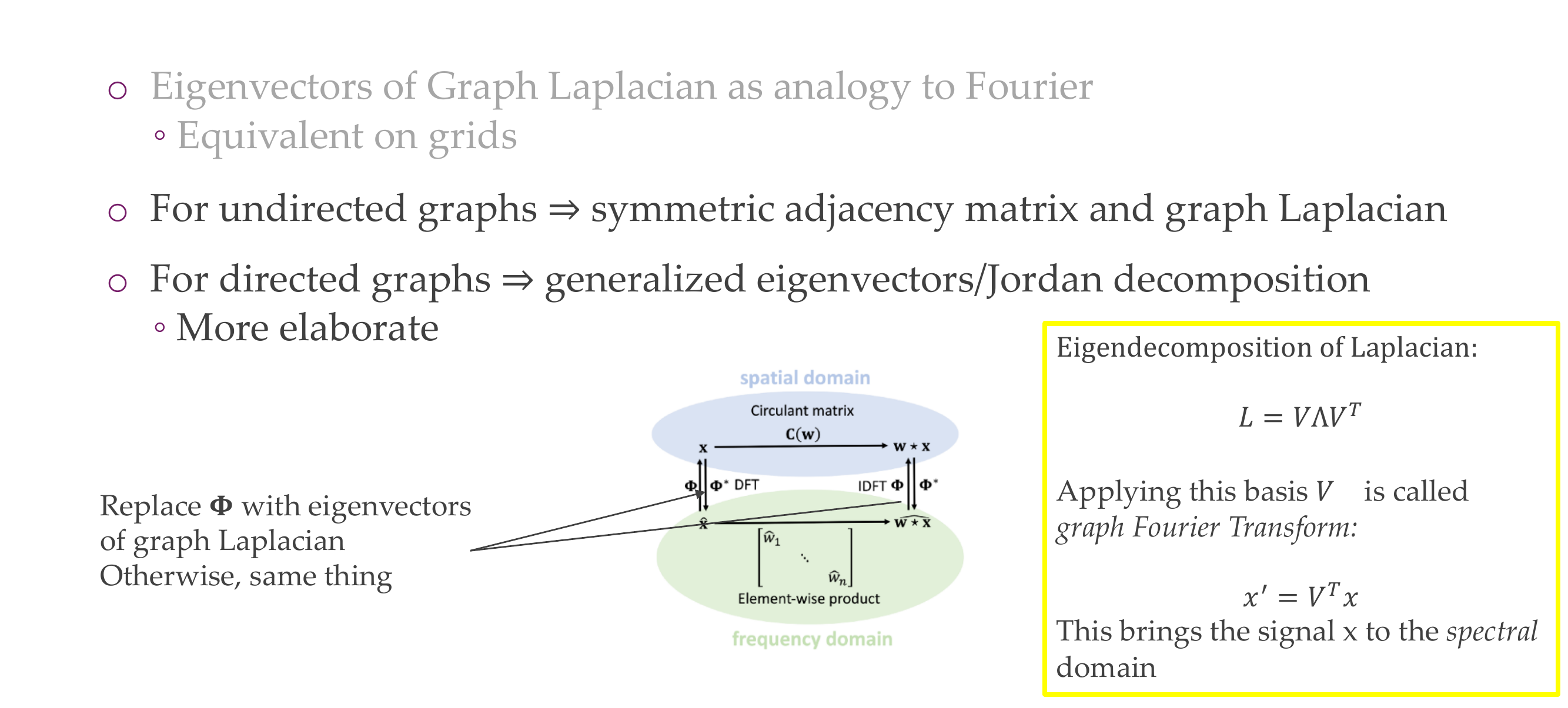
50 Title

Slide 50

51 From convolutions to spectral graph convolutions

Slide 51

52 Approach: Use Eigenvectors of Graph Laplacian to replace Fourier

Slide 52

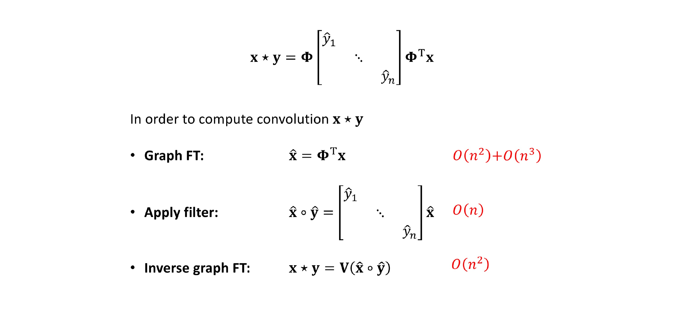
53 Actually:

Slide 53

54 Further details

Slide 54

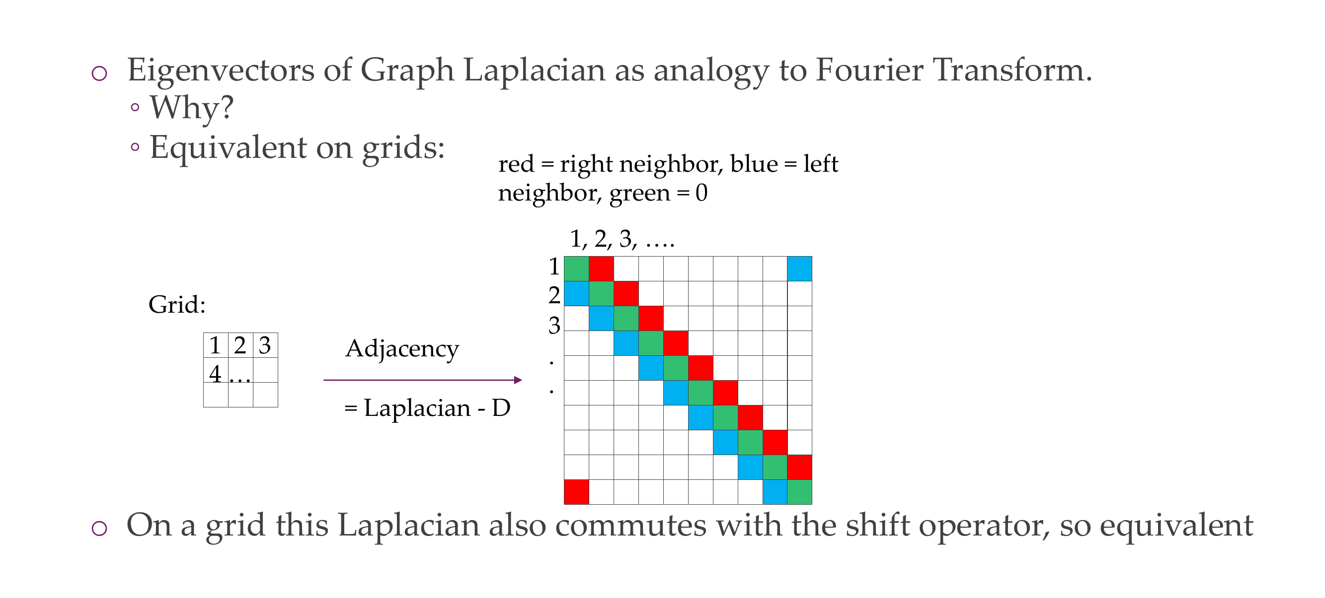
55 In analogy to convolutions in frequency domain:

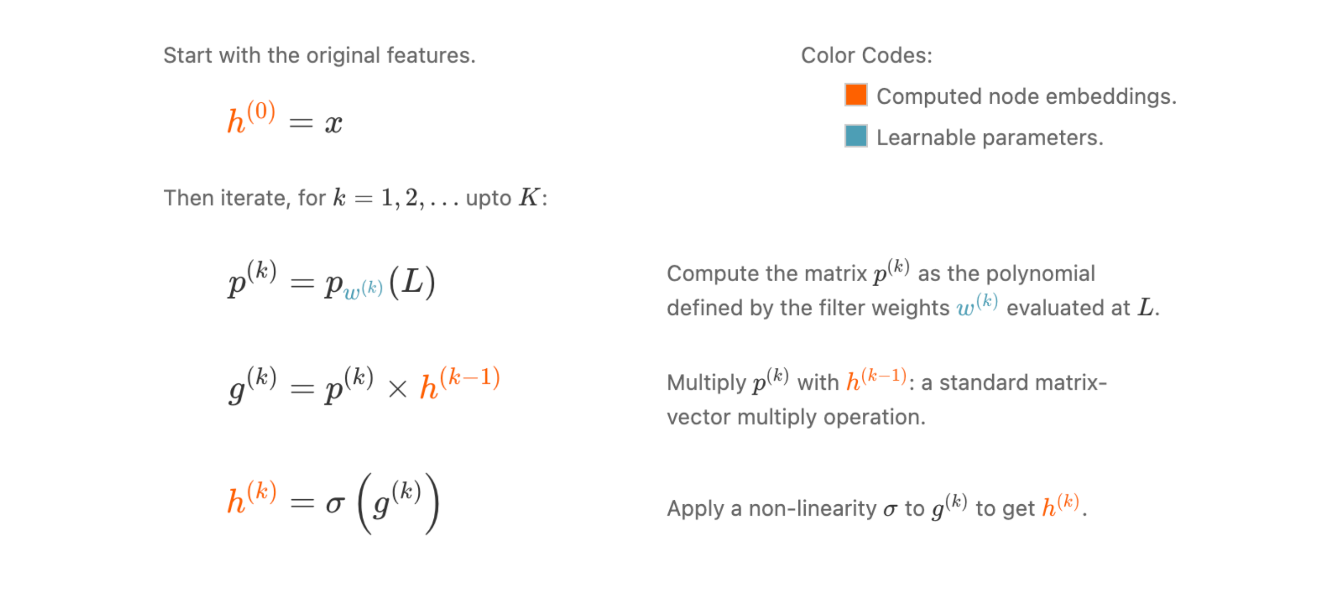
We now define spectral graph convolutions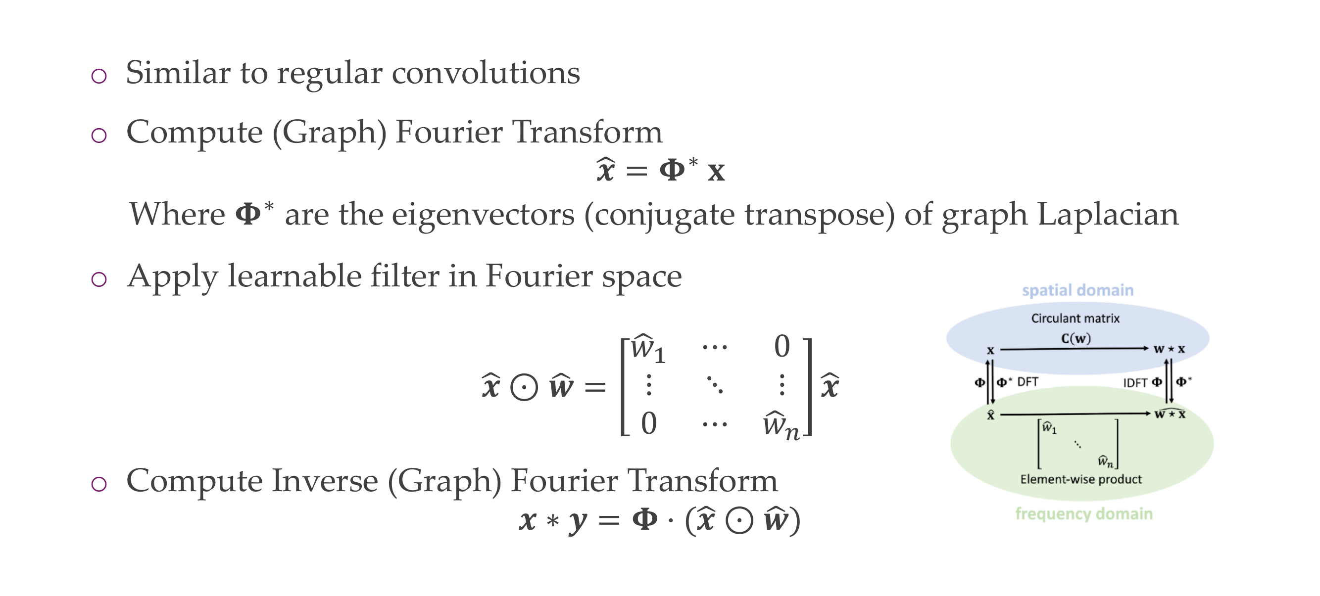

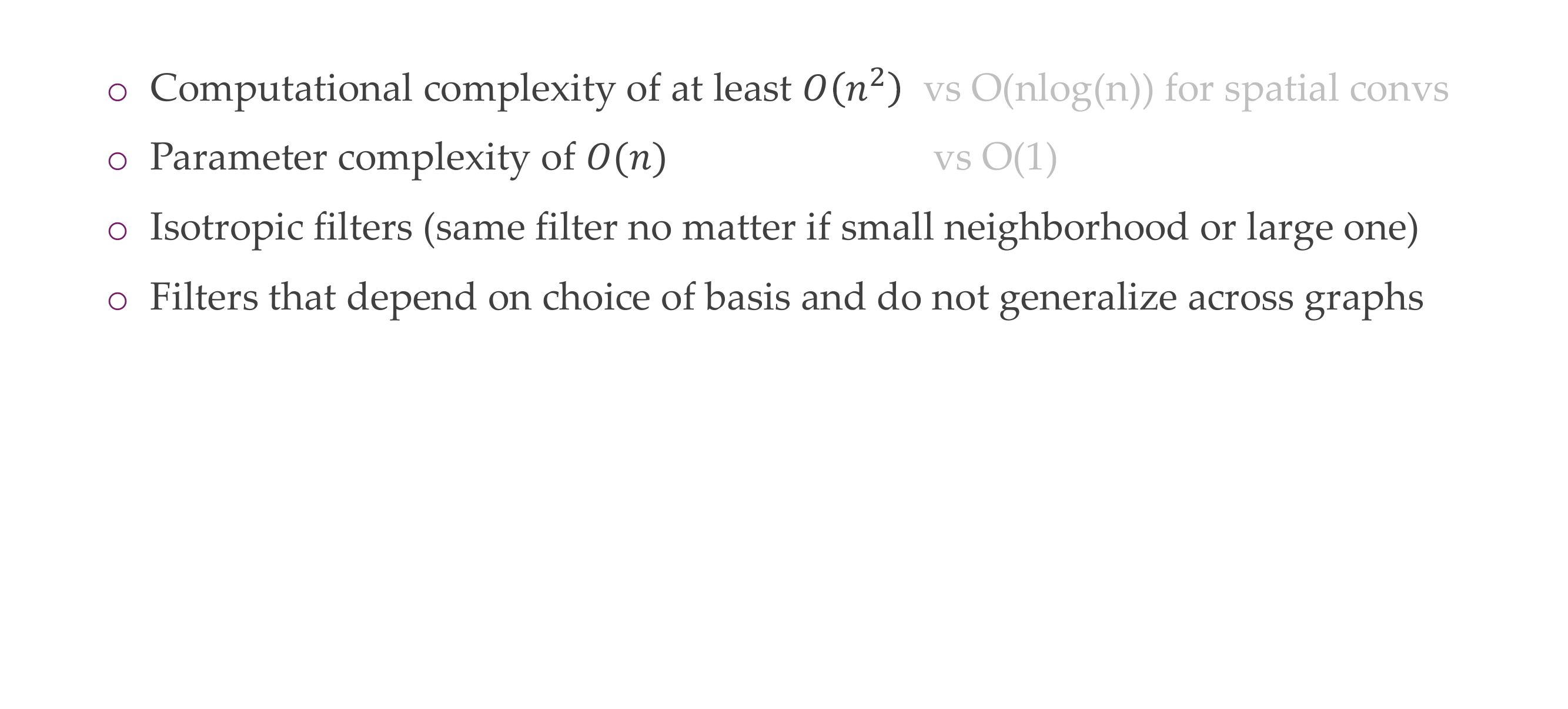
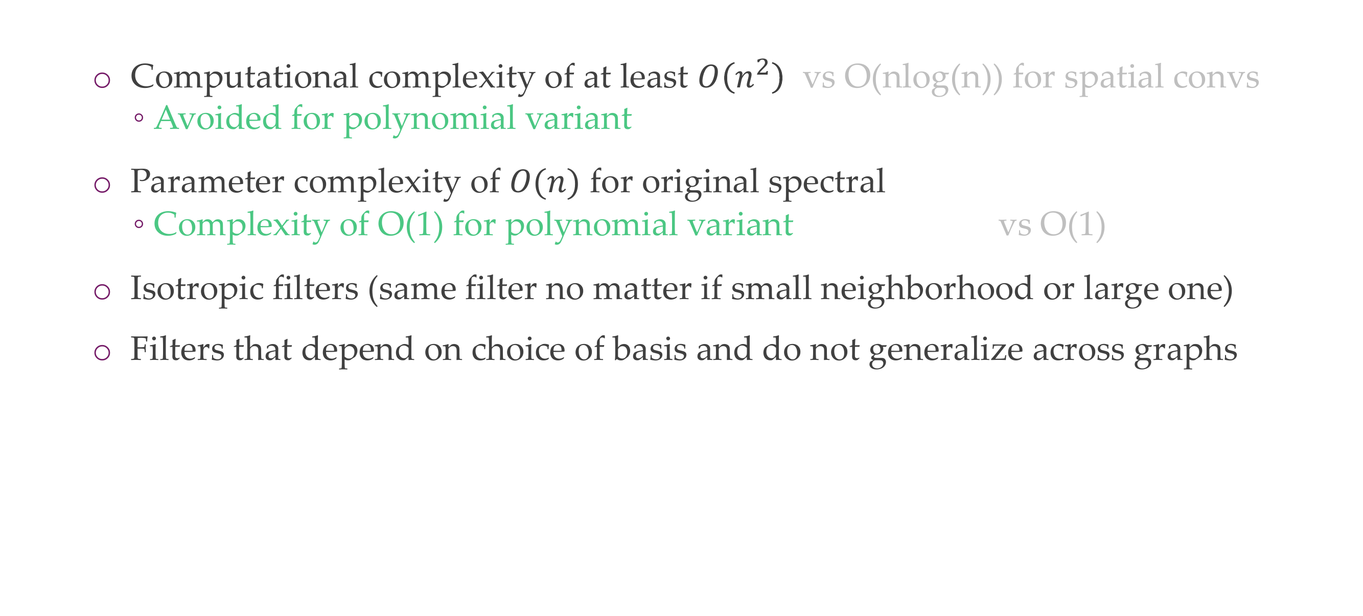
Slide 55

56 Where we are, part 2

Slide 56

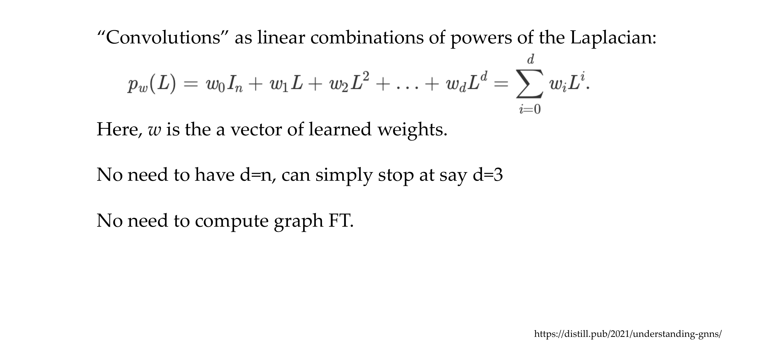
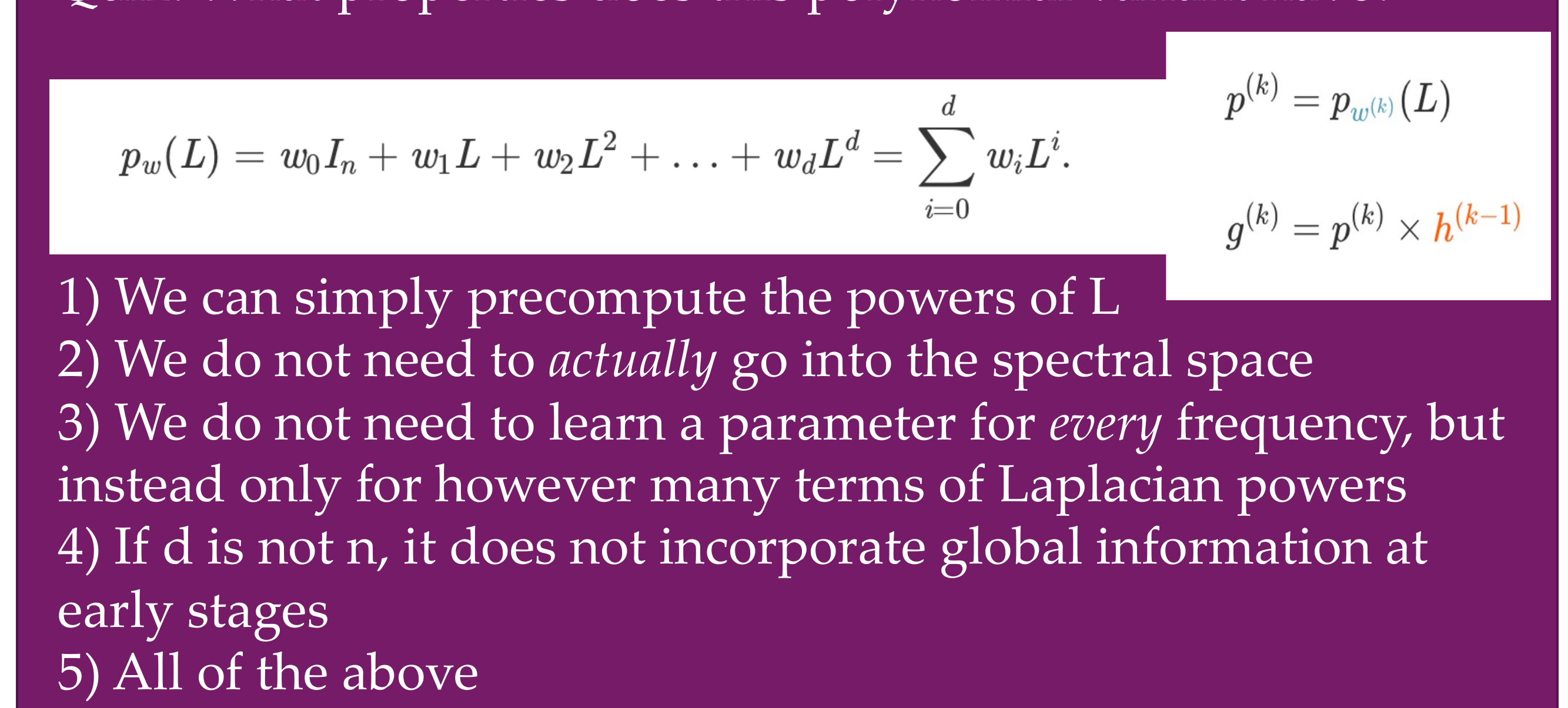
57 Why the graph Laplacian*?

Slide 57

58 Spectral graph convolution

Slide 58

59 Some drawbacks of this variant

Slide 59

60 Easy to increase the field of view with powers of the Laplacian

Slide 60

61 Putting it together: stacking graph convolutions

Slide 61

62 . Quiz: What nronerties does this nolvnomial variant have? |

Slide 62

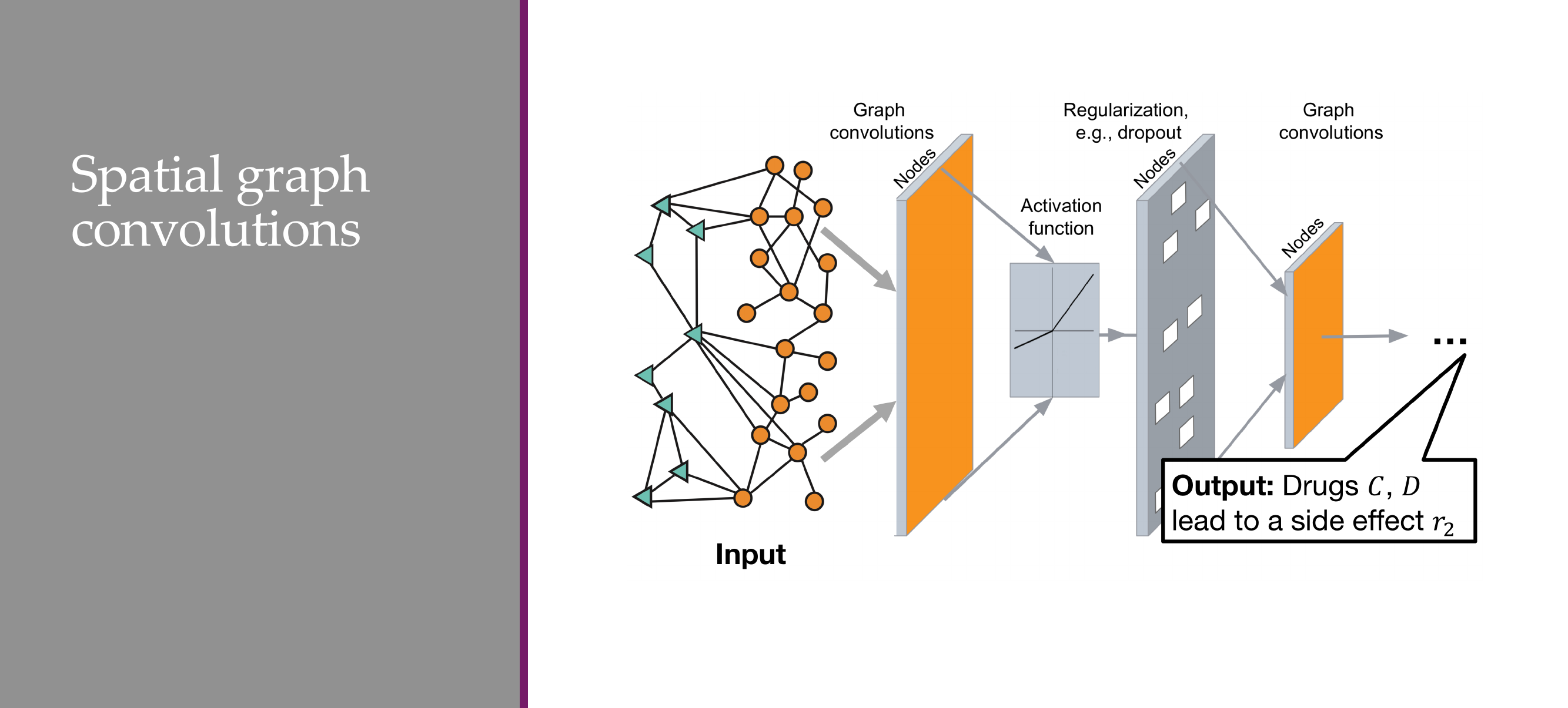
63 Some drawbacks of this variant now

Slide 63

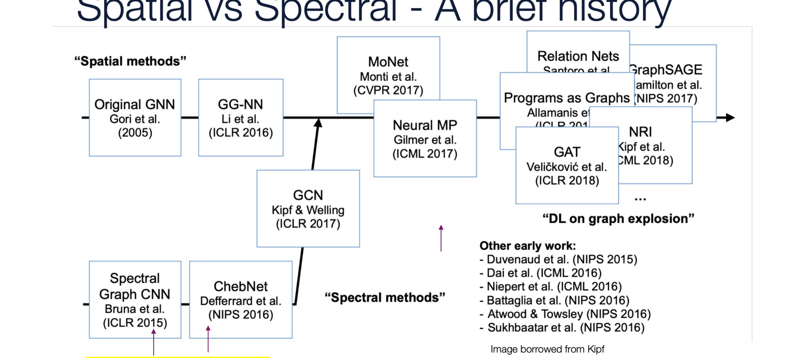
64 Title

Slide 64

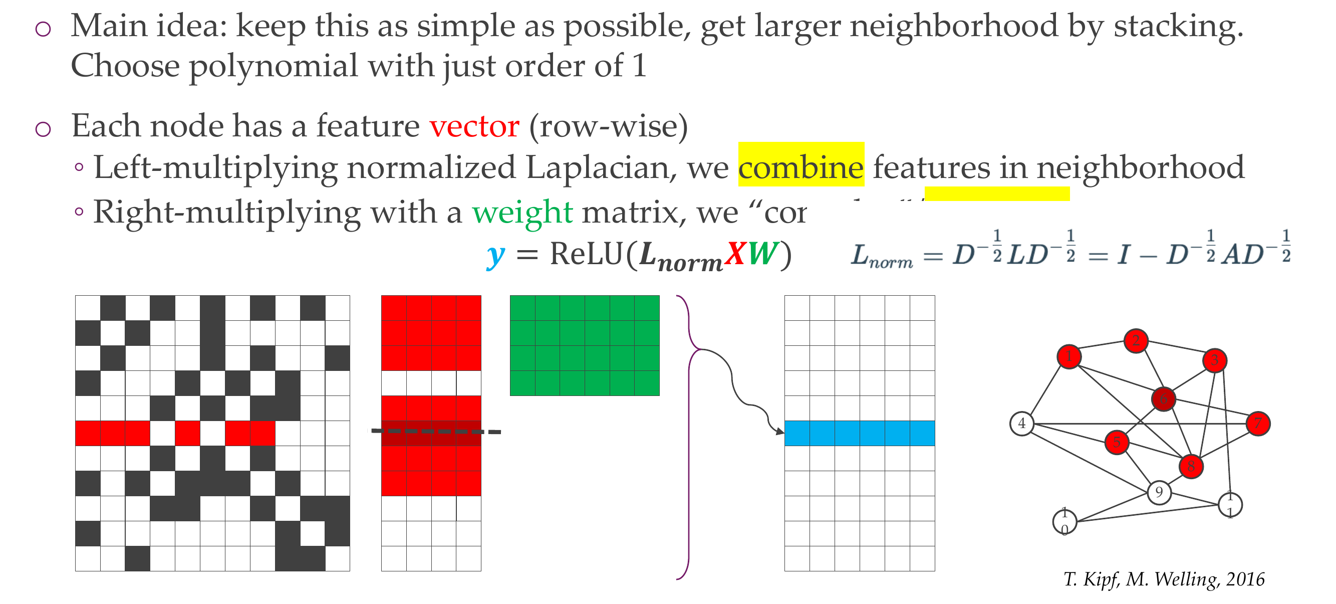
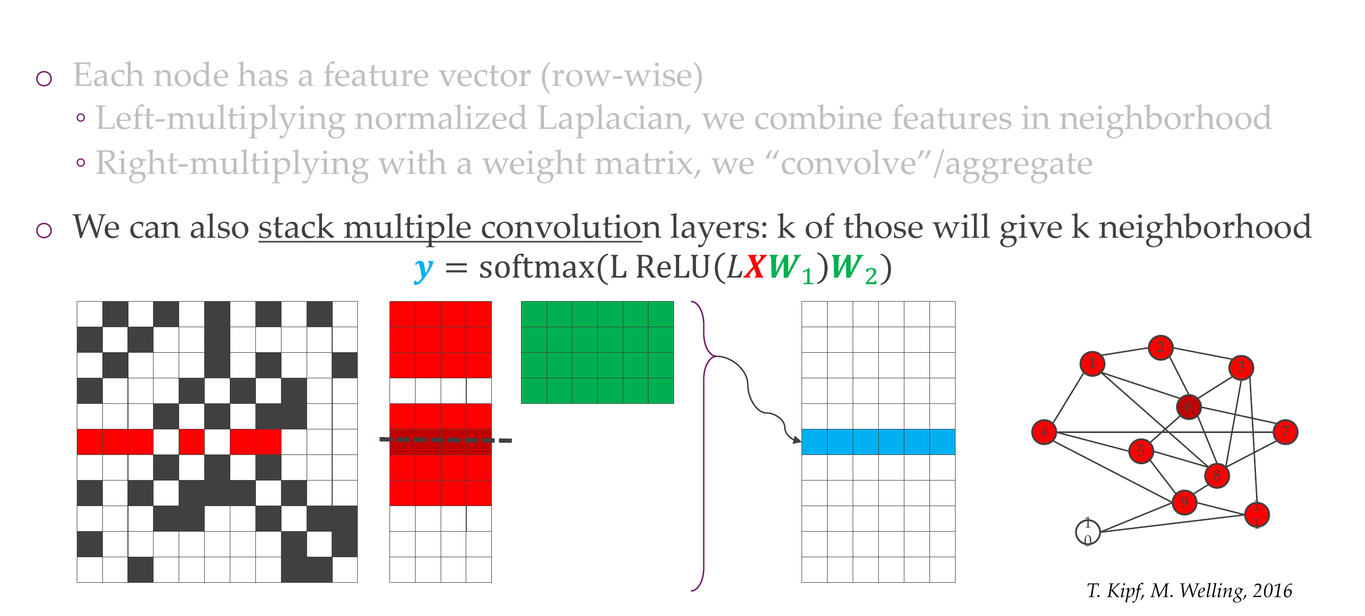
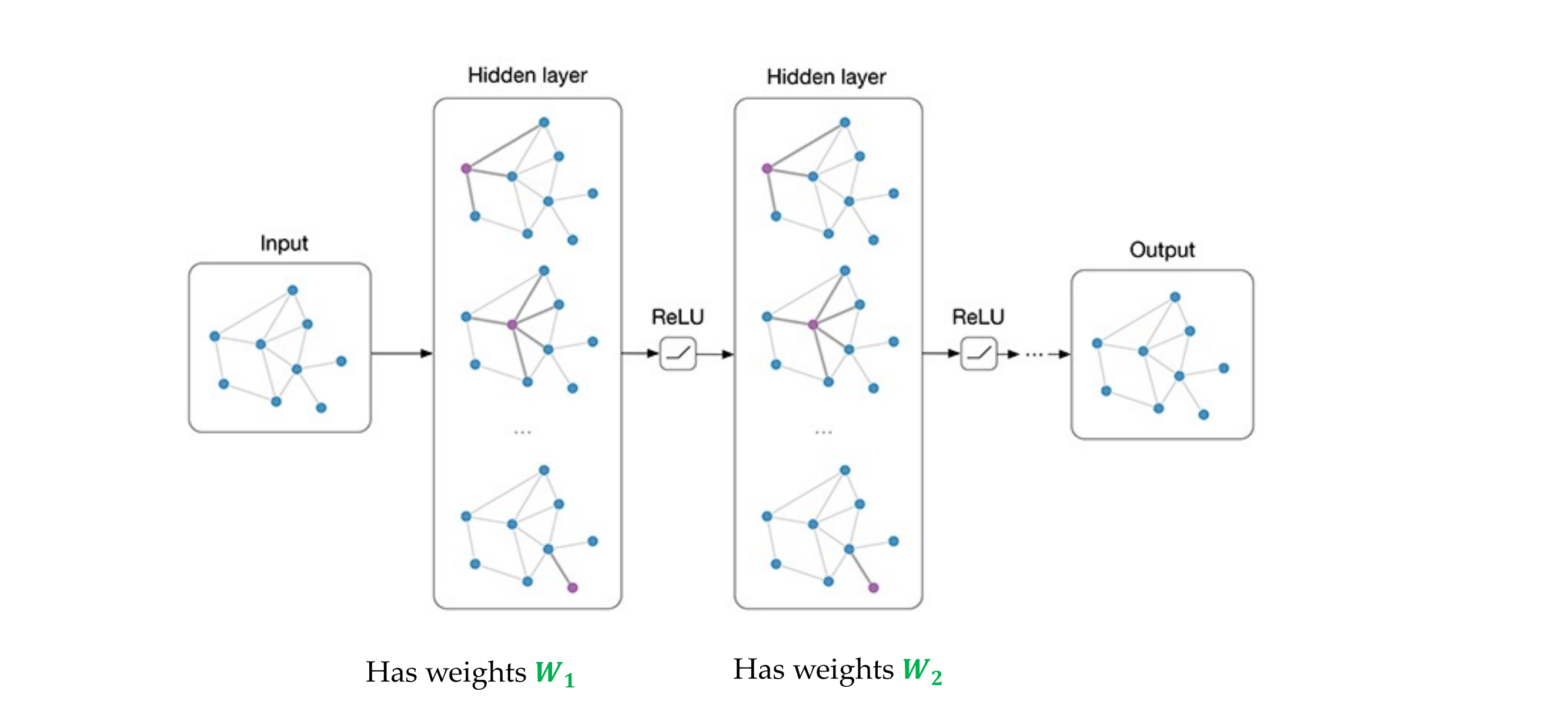
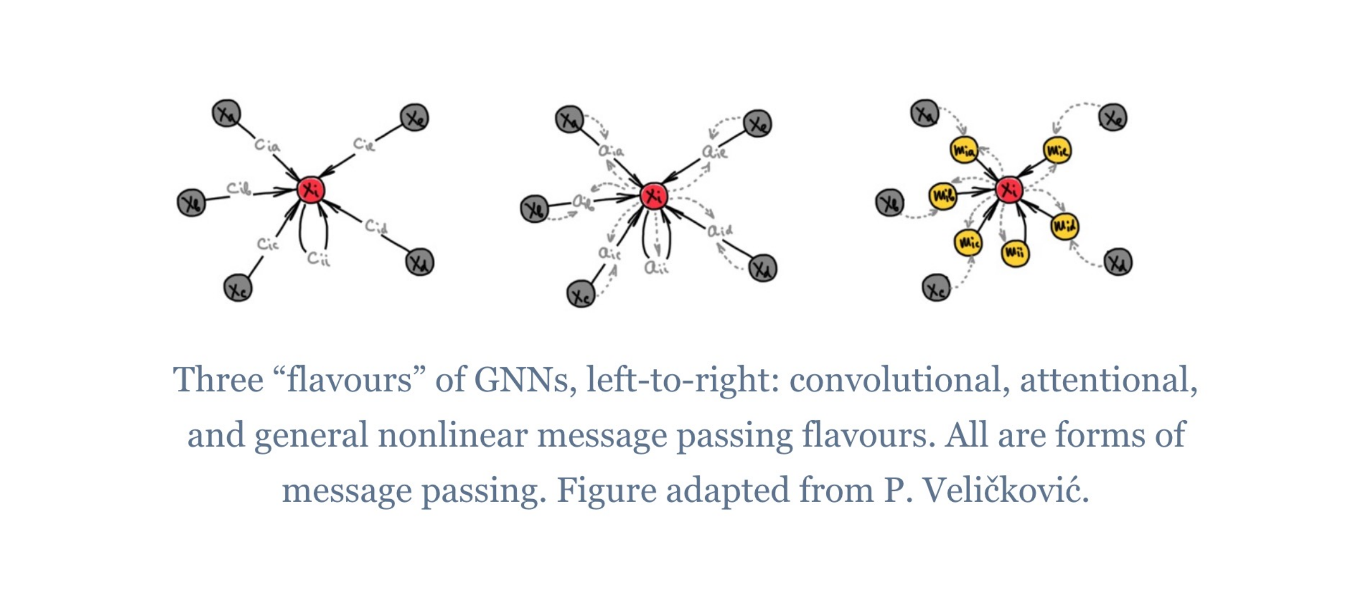
65 A FF fF F Fg

Slide 65

66 Graph convolutions

Slide 66

67 What can we use from the spectral approach?

Slide 67

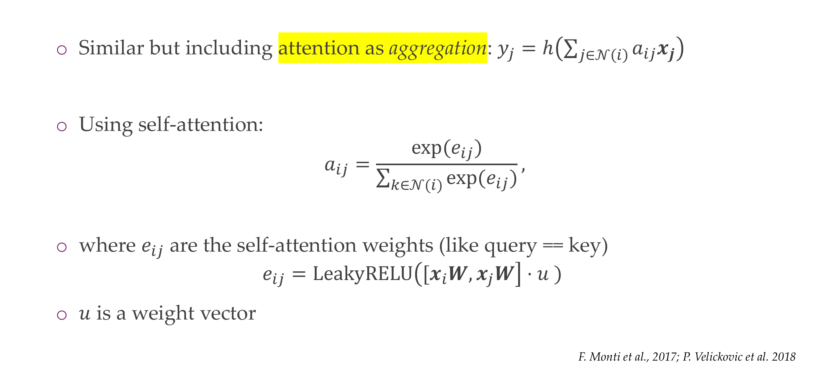
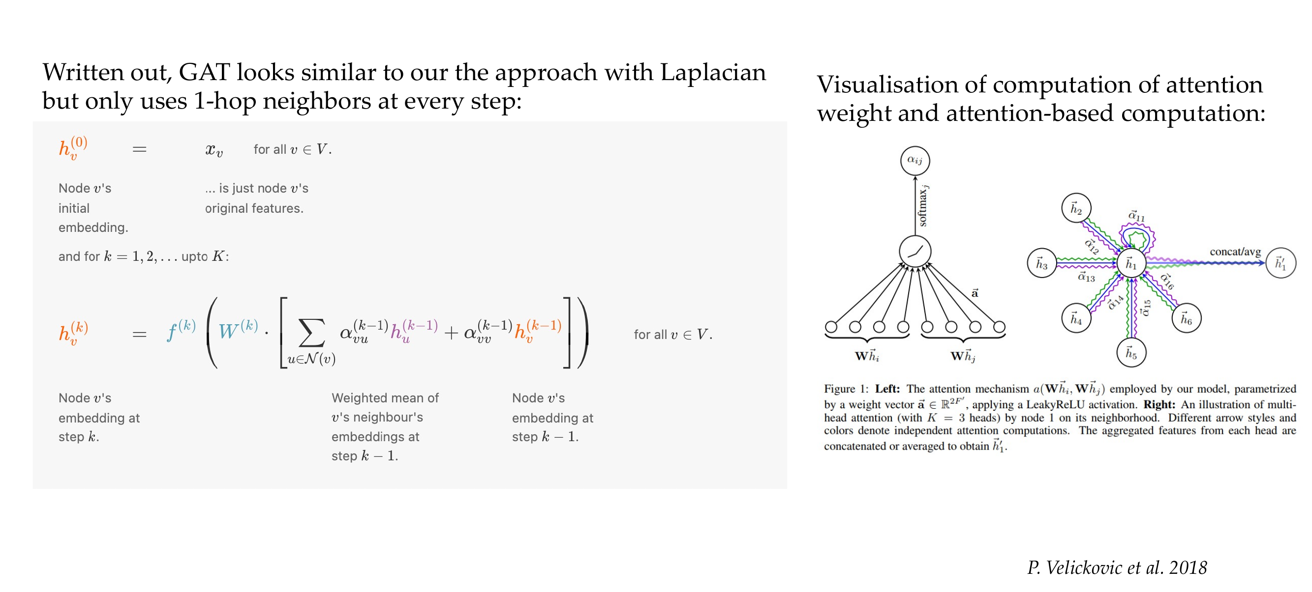
68 Graph Convolutional Networks (GCN)

Slide 68

69 Graph Convolutional Networks (GCN)

Slide 69

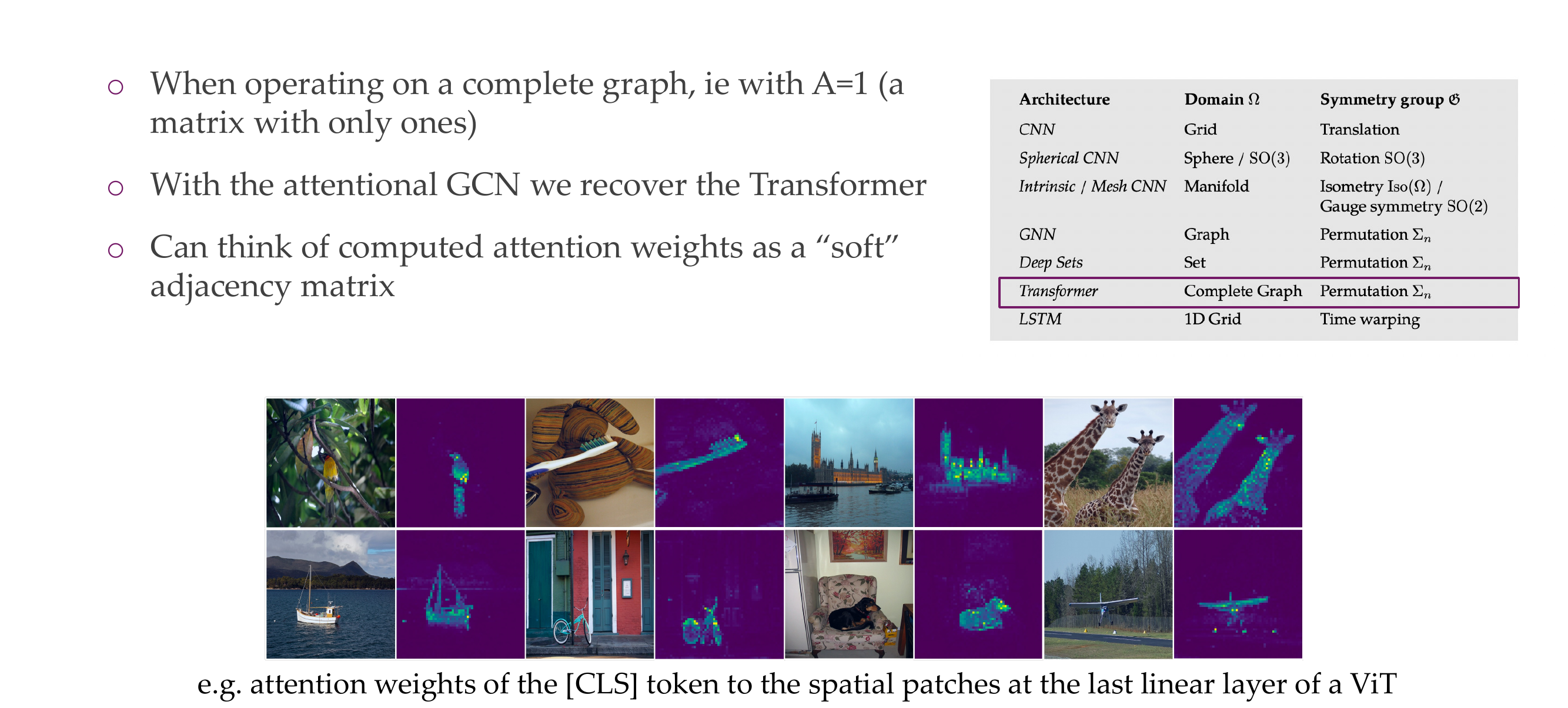
70 Putting it together:

Slide 70

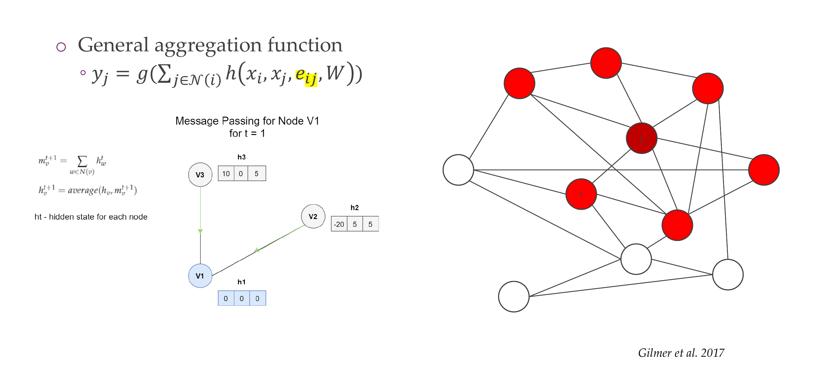
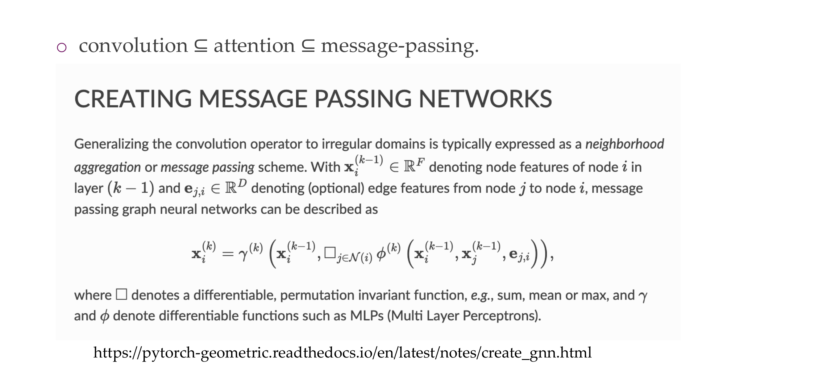
71 Other kind of aggregation: Graph Attention Networks (GAT)

Slide 71

72 Self-attention for graph convolutions

Slide 72

73 Connection to transformers

Slide 73

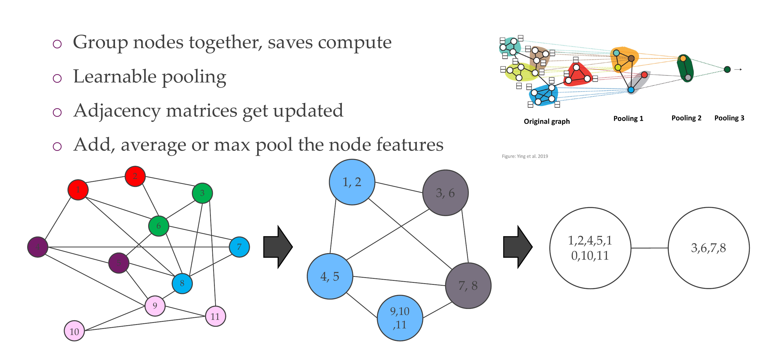
74 Message Passing Neural Network (MPNN)

Slide 74

75 PyTorch Geometric baseclass

Slide 75

76 Overview

Slide 76

77 Finally, a note about coarsening graphs

Slide 77

78 Where we are, part 3

Slide 78

79 The last few lectures

Slide 79

80 Title

Slide 80

81 Title

Slide 81